
What is integration of a single variable?
Earth and Atmospheric Sciences
In the simplest terms, an integral is a mathematical tool used to calculate the “total” of something that is changing or spread out. While basic arithmetic allows you to add up discrete numbers (like 2 + 5), and multiplication helps you find the area of a flat rectangle (length * width), integration allows you to find the area under a curve where the height is constantly shifting.

1. The Geometry Perspective: Area Under a Curve
Imagine you have a curve on a graph. To find the area between that curve and the x-axis, you can’t use a simple formula because the shape isn’t a standard square or circle.
Integration works by slicing that area into an infinite number of incredibly thin vertical rectangles. By adding the areas of all these tiny rectangles together, you get the exact total area of the shape.
2. The Physics Perspective: Accumulation
If you think of a derivative as a “rate of change” (like speed), an integral is the accumulation of that change (like total distance traveled).
- The Derivative: Tells you how fast you are moving at a specific moment.
- The Integral: Tells you how far you have gone over a period of time, even if your speed was constantly changing.
If you have a function representing the flow of water into a tank, the integral of 그 function over time tells you the total volume of water in the tank.

3. The Two Types of Integrals
In calculus, you will encounter two main forms:
- Definite Integrals: These have a specific start and end point (called limits). They result in a single number representing a total value, like an area or a physical quantity.
- Indefinite Integrals: These do not have limits and are often called antiderivatives. They result in a new function that describes the original function’s “parent.”
4. Why the “+ C”?
When you “reverse” a derivative to find an indefinite integral, you include a constant C. This is because when you take the derivative of a constant (like 5 or 100), it becomes zero. When you go backward, you can’t be sure if there was originally a constant there, so the + C acts as a placeholder for any potential constant value.

Real-World Applications
- Engineering: Calculating the center of gravity or the stress on a bridge.
- Biology: Measuring the growth rate of a bacterial population over time.
- Economics: Determining total consumer surplus or the accumulation of capital.
- Data Science: Calculating probabilities (the area under a “bell curve” is an integral).
How can integrals be used to find areas and distances?
Integrating functions allows us to move from a “rate” or a “boundary” to a “total amount.” This process is fundamentally about summation—adding up an infinite number of infinitesimal pieces.
1. Finding Area Under a Curve
In geometry, we have simple formulas for squares or circles, but curves require calculus. The definite integral calculates the area between a function f(x) and the x-axis over an interval [a, b].
- The Concept: We divide the region into rectangles with a width of dx (an infinitely small change in x) and a height of f(x).
- The Math: By summing these rectangles, we get the total area:
- Area Between Two Curves: If you want to find the area trapped between two functions, f(x) and g(x), you subtract the “bottom” function from the “top” function:
2. Finding Distance from Velocity
In physics, distance is the accumulation of speed over time. If you are traveling at a constant 100 km/h for 2 hours, you simply multiply (100 * 2 = 200 km). However, if your speed is constantly changing, you need an integral.
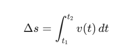
- The Relationship: Velocity v(t) is the derivative of position. Therefore, position is the integral of velocity.
- Total Displacement: This tells you the net change in position from your starting point to your ending point:
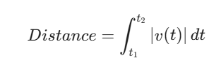
- Total Distance Traveled: Since displacement only cares about the start and end, it can be zero if you return home. To find the actual total distance covered (even if you turned around), you integrate the absolute value of velocity (speed):
3. Summary of the Connection
The “Area” and “Distance” are actually the same concept in different contexts:
| Context | Function | Integral Result |
| Geometry | Height (y) | Total Area |
| Physics | Velocity (v) | Total Distance |
| Statistics | Probability Density | Total Probability |
| Hydrology | Flow Rate | Total Volume of Water |
By finding the area under a velocity graph, you are literally “adding up” every tiny bit of movement that occurred at every fraction of a second.
What is the definite integral?
While an indefinite integral gives you a general formula (a family of functions), a definite integral results in a specific numerical value. It represents the net “accumulation” of a function between two fixed points.
1. The Anatomy of the Definite Integral
It is written with “limits of integration” at the top and bottom of the integral symbol:
- a: The lower limit (where you start).
- b: The upper limit (where you stop).
- f(x): The integrand (the function you are measuring).
- dx: The variable you are integrating with respect to (the “width” of your slices).
2. The Fundamental Theorem of Calculus
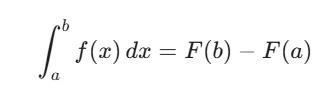
To solve a definite integral, you don’t usually draw rectangles; you use the Fundamental Theorem of Calculus. It bridges the gap between derivatives and integrals:
- Find the antiderivative, F(x).
- Plug in the upper limit (b).
- Plug in the lower limit (a).
- Subtract the two results.
Note: You’ll notice there is no + C in a definite integral. Because you are subtracting F(b) – F(a), the constants cancel out: (F(b) + C) – (F(a) + C) = F(b) – F(a).
3. Geometric Interpretation: Signed Area
A definite integral calculates the signed area between the function and the x-axis.
- Above the x-axis: The area is considered positive.
- Below the x-axis: The area is considered negative.
If a function has equal parts above and below the x-axis between a and b, the definite integral will be zero, even though the “physical” area is larger.
4. Properties of Definite Integrals
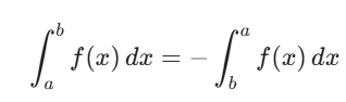
- Order of Limits: If you flip the start and end points, the sign of the result changes:
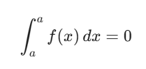
- Zero Width: If the start and end points are the same, the area is zero:
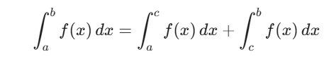
- Additivity: You can split an integral into two parts at any point c in between:
Summary Table: Indefinite vs. Definite
| Feature | Indefinite Integral | Definite Integral |
| Result | A Function (e.g., x2 + C) | A Number (e.g., 25) |
| Limits | None | Lower (a) and Upper (b) |
| Purpose | To find the “parent” function | To find total accumulation/area |
What are area functions and how are they used?
An area function is a specific type of definite integral where the upper limit of integration is a variable rather than a fixed number.
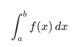
While a standard definite integral like
gives you a single number (the area from 1 to 5), an area function gives you a “sliding” total that changes as you move across the graph.
1. The Mathematical Definition
If f is a continuous function, the area function A(x) is defined as:
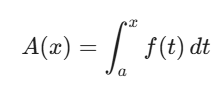
- a: A fixed starting point (the “anchor”).
- x: The independent variable. As x moves, the area grows or shrinks.
- t: A “dummy variable.” We use t inside the integral so it doesn’t get confused with the x used for the upper limit.
2. How Area Functions Work
Think of an area function like a trip odometer in a car.
- The “fixed point” a is where you hit “reset” on your odometer.
- The “function” f(t) is your current speed.
- The “area function” A(x) is the total distance shown on the odometer at any point x along your journey.
As you move x to the right, you are “sweeping out” more area under the curve. If the curve goes below the x-axis, the area function will begin to decrease because you are adding “negative” area.
3. The Second Fundamental Theorem of Calculus
Area functions are the key to understanding one of the most important rules in math. The Second Fundamental Theorem of Calculus states that the derivative of an area function is simply the original function itself:
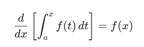
This proves that integration and differentiation are inverse operations. If you accumulate area under a curve (f) to create an area function (A), the rate at which that area grows at any point x is exactly the height of the curve (f(x)) at that point.
4. Practical Uses of Area Functions
Defining New Functions
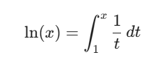
Some functions in science and math cannot be written with basic algebra (like +, -, ×, ÷). We define them using area functions.
- The Natural Logarithm: ln(x) is actually defined as the area under the curve 1/t starting from 1:
- The Error Function (erf): Used in statistics and probability to describe the “bell curve” accumulation.
Accumulation in Physics
In engineering or meteorology, area functions are used to track cumulative totals:
- Precipitation: If f(t) is the rate of rainfall (mm/hr), then A(x) is the total amount of rain that has fallen since the start of the storm up to time x.
- Work: If you are moving an object with a varying force, the area function represents the total work done as a function of the distance traveled.
Solving Differential Equations
Area functions allow us to write solutions for complex systems where we know the “rate of change” but need a formula for the “total amount” at any given time.
What is the Fundamental Theorem of Calculus?
The Fundamental Theorem of Calculus (FTC) is the “bridge” that connects the two main branches of calculus: differential calculus (finding rates of change/slopes) and integral calculus (finding accumulation/area).
Before this theorem was discovered, these two areas were treated as almost entirely separate. The FTC proves that they are inverse operations—much like addition and subtraction.
The theorem is usually divided into two parts.
Part 1: The “Inverse” Relationship
The first part of the theorem states that if you take a continuous function, integrate it to find the area, and then take the derivative of that result, you end up back at the original function.
The Math:
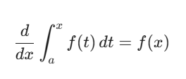
What it means:
It defines an “area function” as the antiderivative of f(x). It essentially says that the rate at which the area under a curve is “growing” at a specific point is equal to the height of the curve at that point.
Part 2: The Evaluation Theorem
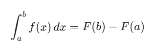
The second part is the practical tool that everyone uses to solve calculus problems. It provides a way to calculate a definite integral without having to add up an infinite number of rectangles (Riemann sums).
The Math:
(Where F is any antiderivative of f.)
What it means:
To find the exact area under a curve between two points a and b:
- Find the antiderivative of the function.
- Plug in the top number (b).
- Plug in the bottom number (a).
- Subtract the results.
Why is this “Fundamental”?
Without the FTC, calculating the area under a curve like y = x2 would require complex limits and massive algebraic summations. The FTC turned a geometric nightmare into a simple subtraction problem.
It allows us to solve massive real-world problems by looking at the “start” and “end” states of a system:
- In Physics: If you know the velocity of a rocket at every second, the FTC lets you find the exact total displacement by simply finding the antiderivative.
- In Engineering: It allows for the calculation of work, energy, and center of mass using simple functional evaluation.
- In Chemistry: It helps determine the total change in concentration of a substance over time based on its reaction rate.
A Simple Analogy
Imagine you are tracking a car’s journey:
- Part 1 says: If you know the total distance traveled at every moment, the “slope” of that distance graph is your speedometer reading (velocity).
- Part 2 says: If you know your velocity at every moment, you can find the total distance you traveled by looking at the change in your “odometer” (the antiderivative) from start to finish.
What is the indefinite integral and what is the Total Change Theorem?
While the definite integral results in a specific number (the area between two points), the indefinite integral and the Total Change Theorem deal with the broader relationship between a rate of change and the original quantity.
1. The Indefinite Integral
The indefinite integral is essentially the process of “undoing” a derivative. If you have a function f(x), the indefinite integral finds the antiderivative—the original function that, when differentiated, would give you f(x).
The Notation
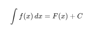
- The instruction to find the antiderivative of whatever is inside.

- f(x): The integrand (the derivative you are starting with).
- F(x): The antiderivative (the “parent” function).
- + C: The Constant of Integration.
Why the + C?
When you take the derivative of a constant (like 5 or -12), it becomes 0. Therefore, if you are working backward from a derivative, you have no way of knowing if the original function had a constant attached to it.
- If F(x) = x2 + 10, the derivative is 2x.
- If F(x) = x2 – 50, the derivative is also 2x.To account for every possible original function, we add + C.
2. The Total Change Theorem
The Total Change Theorem is a specific application of the Fundamental Theorem of Calculus. It states that the integral of a rate of change is the total change in the original quantity over a specific time interval.
The Formula
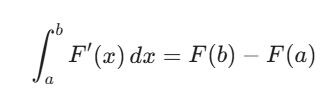
In plain English: If you add up all the tiny changes (F'(x)) between point a and point b, you get the net difference in the value of the function (F) at those two points.
3. Real-World Applications
This theorem is the foundation for solving problems in science and economics where we only know how fast something is changing, but we need to know the final result.
| If the Integrand is… | The Total Change Theorem gives you… |
| Velocity (v(t)) | Displacement: The change in position from $a$ to $b$. |
| Current (I(t)) | Charge: The total electrical charge that passed through a wire. |
| Birth Rate (B(t)) | Population Growth: The net increase in people over a decade. |
| Marginal Cost (C'(x)) | Total Cost Increase: The cost of increasing production from $a$ to $b$ units. |
| Precipitation Rate | Accumulated Rainfall: The total depth of water after a storm. |
Example: A Leaking Tank
If a tank is leaking water at a rate of r(t) liters per minute, and you want to know how much water was lost between the 10th and 20th minute, you integrate the rate:
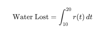
The result isn’t just a mathematical area; it is the physical volume of water that left the tank.
Who invented calculus and why this fight between the Germans and the British?
The “Calculus Wars” are one of the most famous and bitter disputes in the history of science. While both men reached the finish line around the same time, they took very different paths to get there.
The Two Contenders
1. Sir Isaac Newton (The British Side)
Newton began developing his “Method of Fluxions” in the mid-1660s while Cambridge was closed due to the Great Plague.
- His Approach: Newton’s calculus was rooted in physics and motion. He thought of curves as the path of a moving point and derivatives as “velocities.”
- The Delay: Newton was notoriously private and terrified of criticism. He used calculus to prove the laws of planetary motion in his masterpiece, Principia Mathematica (1687), but he didn’t explicitly explain the method of calculus until much later.
2. Gottfried Wilhelm Leibniz (The German Side)
Leibniz developed his version of calculus independently in the mid-1670s.
- His Approach: Leibniz’s calculus was rooted in philosophy and logic. He saw integration as a sums of infinitesimal areas.
- The Publication: Unlike Newton, Leibniz published his work quickly, in 1684. Most importantly, he invented the notation we still use today, such as the integral symbol ($\int$) and the $dy/dx$ notation for derivatives.
Why the Fight?
The dispute wasn’t just about math; it was about national pride and intellectual property.
1. The Accusation of Plagiarism
In the late 1690s, friends of Newton began suggesting that Leibniz had seen Newton’s private papers during a visit to London in 1676 and “stole” the idea. Leibniz was outraged, as he had arrived at his conclusions through a completely different logical path.
2. The Royal Society “Investigation”
Leibniz eventually appealed to the Royal Society in London to clear his name. However, Newton was the President of the Royal Society.
- Newton hand-picked the committee to “investigate” the claim.
- Newton secretly wrote the final report himself, which—unsurprisingly—concluded that Leibniz was a plagiarist.
3. The Consequences
The fallout was devastating for European mathematics:
- British Isolation: British mathematicians stubbornly stuck to Newton’s clunky notation ($\dot{x}$) out of loyalty. Because of this, they fell behind for nearly a century.
- Continental Progress: Mathematicians in mainland Europe (like the Bernoulli brothers) used Leibniz’s more flexible notation, which allowed them to make rapid advancements in physics and engineering.
The Verdict of History
Today, historians agree on Independent Discovery.
- Newton was likely the first to invent it (around 1665).
- Leibniz was the first to publish it (1684) and gave us the superior mathematical language to use it.
Modern calculus is effectively a “Leibnizian” system used to solve “Newtonian” problems. We use Leibniz’s symbols to calculate the physics Newton described.
What is the substitution rule?
The Substitution Rule (often called u-substitution) is essentially the “Chain Rule in reverse.”
In differentiation, the Chain Rule handles functions nested inside other functions. In integration, u-substitution allows you to simplify a complex integral by changing the variable, making it look like a basic standard integral.
1. The Core Concept
The goal is to replace a piece of the integral with a new variable, usually $u$. This is effective when you notice that one part of the function is the derivative of another part of the function.
If you have an integral in the form:
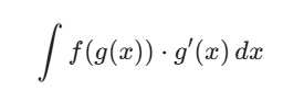
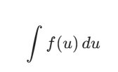
You can set u = g(x). This means that the derivative du is g'(x)dx. The integral then simplifies to:
2. The Step-by-Step Process
To solve an integral using substitution, follow these four steps:
- Choose u: Look for an “inner” function whose derivative also appears in the integral.
- Compute du: Take the derivative of u with respect to x and solve for dx.
- Substitute: Replace all x terms and the dx with u and du. (Crucial: No x terms should remain).
- Integrate and Back-Substitute: Solve the simpler integral in terms of u, then replace u with the original x expression.
3. Example in Action
Suppose you want to find:
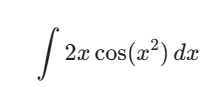
- Step 1: Notice that x2 is inside the cosine, and its derivative (2x) is sitting right outside. Let u = x2.
- Step 2: Then du = 2xdx.
- Step 3: Substitute into the integral:
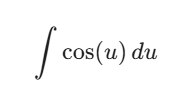
- Step 4: Integrate: sin(u) + C.
- Back-Substitute: Replace u with x2. Result: sin(x2) + C
4. Substitution with Definite Integrals
When dealing with a definite integral (one with limits a and b), you have two choices:
- Option A: Ignore the limits, integrate using u, back-substitute to x, and then apply the original limits.
- Option B (Preferred): Change the limits of integration to match u immediately. If u = g(x), then the new limits are g(a) and g(b).

Why it Matters
Substitution is one of the most powerful tools in a calculus toolkit. It allows you to transform “messy” real-world data—like varying atmospheric pressure or fluctuating electrical signals—into clean, solvable mathematical models.