Calculus I – Differentiation of a Single Variable

What are the four ways to represent a function?

At its simplest, a mathematical function is a rule that takes an input, processes it, and delivers a unique output. Think of it as a predictable machine: you drop an input (x) into the slot, the machine applies its specific rule (f), and it spits out a single, definitive result (y).

Mathematically, we write this as:

Where functions get incredibly powerful is when we use them to model the world. Modeling is the process of translating real-world behavior into mathematical equations so we can understand, predict, and control them.

How Functions Map to Reality

To model something, we look for cause-and-effect relationships. The “cause” is our independent variable (the input), and the “effect” is our dependent variable (the output).

Here is how different types of functions capture different slices of reality:

Constant Growth and Decay (Linear Functions)

Linear functions model scenarios where something changes at a steady, unchanging rate.

• The Math: f(x) = mx + b
• The Real World: Think of a water reservoir emptying at a constant rate, or converting Celsius to Fahrenheit. If you travel at a constant speed of 80 km/h, your distance (d) as a function of time (t) is modeled by d(t) = 80t.

Acceleration and Gravity (Quadratic Functions)

When rates of change are themselves changing, linear functions aren’t enough. Quadratic functions capture acceleration, curved trajectories, and optimization.

• The Math: f(x) = ax² + bx + c
• The Real World: When you toss a ball into the air, gravity pulls it back down. Its height over time forms a parabola. Engineers use quadratic models to determine the optimal shape of satellite dishes or to calculate the maximum load a bridge can sustain.

Rapid Scaling (Exponential Functions)

Exponential functions model systems where the amount of growth depends directly on the current size of the population or quantity. The larger it gets, the faster it grows (or decays).

• The Math: f(x) = ab^x
• The Real World: This is how we model the spread of a virus, compound interest in a bank account, or the radioactive decay of elements deep inside the Earth.

Rhythms and Cycles (Trigonometric Functions)

Many things in nature don’t grow forever; they repeat. Trigonometric functions (like sine and cosine waves) are perfect for capturing cyclic patterns.

• The Math: f(x) = Asin(Bx – C) + D
• The Real World: Ocean tides, sound waves, alternating electrical current (AC), and seasonal temperature fluctuations are all modeled using periodic functions.

Why Do We Model?

We don’t just build these models for fun; they are foundational to science, engineering, and economics for three main reasons:

• Prediction (Extrapolation): If a function accurately models a planet’s orbit, astronomers can predict exactly where that planet will be 500 years from now, or when the next solar eclipse will occur.
• Understanding History (Interpolation): Models allow us to fill in the blanks where data is missing. By fitting a function to existing climate data, scientists can estimate global temperatures from eras before modern thermometers existed.
• Optimization: Functions allow us to find the “sweet spot.” An aerospace engineer can use a function representing air resistance to find the exact shape of a rocket hull that minimizes drag and maximizes fuel efficiency.

Every smartphone app, weather forecast, video game physics engine, and economic policy relies on networks of these mathematical functions acting as blueprints for reality.

What are mathematical models?

At its core, a mathematical model is a translation of a real-world system into the language of mathematics. It uses equations, variables, and geometric structures to mimic how something behaves in real life so that we can study it, run simulations, and predict future outcomes without having to physically build or manipulate the system itself.

If reality is too messy, dangerous, or massive to experiment on directly, a mathematical model acts as a pristine, digital sandbox.

The Anatomy of a Model

Every mathematical model is built from three fundamental building blocks:

• Variables: The changing quantities within the system.
  • Independent variables (inputs like time or temperature).
  • Dependent variables (outputs like population size or structural strain).
  • State variables (the internal status of the system).
• Parameters: The constants that define the specific conditions of the environment. For example, if you are modeling a falling object, the acceleration due to gravity (g) is a parameter. If you change locations to Mars, the model stays the same, but the parameter changes.
• Functional Relationships: The mathematical rules (equations, inequalities, or differential equations) that dictate exactly how the variables and parameters interact with one another.

The Mathematical Modeling Cycle

Creating a model isn’t a one-time calculation; it is an iterative loop. It bridges the gap between abstract math and concrete reality through a systematic process:

1. Identify & Simplify: Look at a complex real-world problem and strip away the noise. (e.g., If modeling a car’s trajectory, you might initially ignore air resistance and treat the car as a single point mass).
2. Formulate: Translate the simplified reality into mathematical expressions. This is where you define your equations, like using Newton’s Second Law: F = ma
3. Solve: Use algebraic manipulation, calculus, or computer algorithms to solve the equations and see what the math predicts.
4. Interpret: Translate those mathematical solutions back into real-world terms. (e.g., “The math says the rocket will land at coordinate X after T seconds.”)
5. Validate & Refine: Compare the model’s predictions against actual experimental data. If the prediction matches reality, the model is viable. If it fails, you go back to step one, add back some of the complexity you ignored (like air resistance), and refine the equations.

Common Types of Models

Depending on what you are trying to capture, models generally fall into a few distinct categories:

Deterministic vs. Stochastic (Probabilistic)

• Deterministic: Models where the outcomes are precisely determined through known relationships, with no room for random chance. If you input the same data twice, you get the exact same output every time (e.g., calculating the trajectory of a spacecraft).
• Stochastic: Models that account for randomness, unpredictable fluctuations, and probabilities. Instead of giving a single definitive answer, they provide a range of likely outcomes (e.g., stock market projections or predicting the spread of a wildfire based on shifting wind patterns).

Static vs. Dynamic

• Static: Captures a system at a single fixed point in time, like a structural blueprint calculating the weight distribution on a bridge’s support beams.
• Dynamic: Accounts for time-dependent changes, tracking how a system evolves over a continuous timeline, like modeling fluid dynamics in a pipe or population shifts in an ecosystem.

Real-World Impact

Mathematical models are the hidden infrastructure powering the modern world. They are used to build the physics engines in video games, optimize supply chains for global shipping companies, train machine learning algorithms, and map the long-term effects of climate change. Ultimately, a model is only as good as its assumptions—but when designed well, it gives us the power to see into the future of a system before that future even happens.

How can new functions be made from old functions?

Just like building complex structures out of standard Lego blocks, mathematicians and software engineers rarely build complex functions from scratch. Instead, they take basic, well-understood “parent” functions—like linear, quadratic, or trigonometric functions—and combine or modify them to create entirely new behaviors.

There are four primary ways to manufacture new functions from old ones: arithmetic operations, composition, transformations, and piecewise construction.

Algebraic Operations (Combining Them)

The most straightforward way to create a new function is to take two existing functions, f(x) and g(x), and combine them using basic arithmetic.

If you have two functions acting on the same input domain, you can add, subtract, multiply, or divide them:

• Sum: (f + g)(x) = f(x) + g(x)
• Difference: (f – g)(x) = f(x) – g(x)
• Product: (f × g)(x) = f(x) × g(x)
• Quotient: (f/g)(x) = f(x)/g(x) (where g(x) ≠ 0)

Real-World Example: If R(t) represents a company’s revenue over time and C(t) represents its operating costs, you can subtract the two old functions to create an entirely new profit function:

$$P(t) = R(t) – C(t)$$

Composition (Chaining Them)

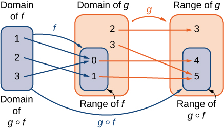
Function composition is the process of plugging one function directly into another. Instead of evaluating them separately, the output of the first function (g) becomes the raw input for the second function (f).

This is written as (f ∘ g)(x), which is read as “f of g of x”:

Think of it like an assembly line: Input $x$ goes into machine g, machine g processes it into an intermediate product, and then machine f takes that product and finishes the job.

Real-World Example: Suppose the number of bacteria in a food item depends on its temperature, N(T), and the temperature of that food depends on how many hours it has been sitting out of the fridge, T(h). By composing them, you get a new function N(T(h)) that tells you the bacteria count directly based on the number of hours elapsed (h).

Transformations (Tweaking Them)

If you already have a function that behaves roughly the way you want, but it’s in the wrong position or scales too slowly, you can apply transformations. By adding, subtracting, or multiplying constants directly to the input or output, you can shift, stretch, or flip the graph of the function.

Given a parent function f(x), a transformed function g(x) looks like this:

Here is how those added parameters alter the old function:

• Vertical Shifting (d): Adding d moves the entire function up or down.
• Horizontal Shifting (c): Subtracting c shifts the function left or right.
• Vertical Stretching/Compressing (a): Multiplying the outside by a changes the amplitude or height. If a is negative, it reflects the function upside down across the x-axis.
• Horizontal Stretching/Compressing (b): Multiplying the input variable by b speeds up or slows down how quickly the function progresses across the x-axis.

Piecewise Construction (Stitching Them Together)

Sometimes, a single mathematical rule can’t capture a real-world scenario across an entire timeline or range. In this case, you can create a piecewise function by taking snippets of different old functions and assigning them to specific intervals.

This creates a brand new behavior by forcing the system to switch rules depending on what the current input value is.

Real-World Example: Tax brackets are classic piecewise functions. Your tax rate stays constant (a linear function) up to a certain income threshold, and the moment your income crosses that boundary, the model switches to a steeper linear function for the next interval of earnings.

What are the strengths and weaknesses of graphing calculators and computers?

When it comes to visualizing functions and executing mathematical models, both graphing calculators and computers are essential tools, but they are built for entirely different environments.

Here is a breakdown of how they stack up against each other in terms of strengths and weaknesses.

Graphing Calculators (e.g., TI-84, TI-Nspire, Casio)

Graphing calculators are dedicated, single-purpose devices. While they might seem like a throwback to an earlier era of technology, they remain a staple in mathematics education for very specific reasons.

Strengths

• Exam-Sanctioned: Their biggest advantage is that they are universally permitted on major standardized tests (like the SAT, AP, and IB exams). Because they lack internet access, they are trusted by testing boards.
• Distraction-Free: Without notifications, social media, or open web browsers, they force total focus on the mathematics at hand.
• Durability and Battery Life: They are built like bricks and can often run for weeks or months on a single charge or a set of AAA batteries.
• Tactile Reliability: Physical buttons make it easy to enter formulas rapidly without relying on a touchscreen or an on-screen keyboard.

Weaknesses

• Outdated Hardware for the Price: Compared to modern smartphones and laptops, graphing calculators have low-resolution screens, sluggish processors, and incredibly limited memory, despite often costing over $100.
• Clunky User Interface: Navigating menus, typing out letters, and adjusting window boundaries (X_min, X_max) requires tedious multi-button sequences.
• Static Graphics: The graphs are typically static. While newer models have color screens, they lack the smooth, fluid, real-time rendering of modern web applications.

Computers (Laptops, Tablets, and Desktops)

Computers leverage massive processing power and an endless ecosystem of software—ranging from intuitive web apps like Desmos and GeoGebra to heavy-duty programming environments like MATLAB, R, and Python.

[Image comparing a traditional graphing calculator screen with a modern computer-based dynamic graphing software interface]

Strengths

• Immense Processing Power: Computers can handle massive datasets, execute complex simulations, and render intricate 3D models instantaneously.
• Dynamic and Interactive UIs: Software like Desmos allows you to add sliders to variables, letting you watch a function transform in real time as you adjust a parameter.
• Versatility and Scale: You aren’t locked into a proprietary system. You can easily export graphs into research papers, write custom code to model unique scenarios, or pull live data from the internet.
• Cost-Efficiency: While a computer itself is an investment, the best mathematical graphing and modeling tools available on them (like Python or web-based calculators) are completely free.

Weaknesses

• The Distraction Factor: A computer is a gateway to the entire internet. It takes significantly more discipline to stay on task when a browser tab can instantly pivot to games, videos, or messages.
• Prohibited in Testing: Because computers can connect to the internet, run unauthorized scripts, or access AI tools, they are strictly banned from almost all formal math examinations.
• Steep Learning Curves: While basic web tools are user-friendly, professional modeling software (like MATLAB or Python data science libraries) requires learning syntax and programming concepts before you can even plot a basic curve.

Summary Comparison

Feature	Graphing Calculator	Computer / Laptop
Primary Use Case	Classroom learning & formal exams	Professional modeling, research, & homework
Portability & Battery	High portability, massive battery life	Moderate portability, requires frequent charging
Visual Quality	Low-res, often pixelated	High-res, dynamic, 3D capable
Data Capacity	Tiny (kb to mb of storage)	Virtually unlimited (gb to tb of storage)
Input Method	Dedicated physical keypad	Keyboard, mouse, or touchscreen

Can artificial intelligence assist in finding the nature of a function that graphing calculators and computers cannot?

Yes, absolutely. To understand how, it helps to draw a line between traditional computer software (like Computer Algebra Systems, or CAS) and modern Artificial Intelligence.

Traditional computers and graphing calculators are strictly deductive. If you give them a precise mathematical rule, they can execute it, plot it, or manipulate it flawlessly. However, if you give them a massive, chaotic mess of real-world data and ask, “What is the underlying mathematical nature of the function that generated this?”, they often hit a wall.

Artificial intelligence is inductive. It excels at pattern recognition, intuition, and searching massive hypothesis spaces. Here is how AI uncovers the nature of functions in ways traditional computing tools cannot:

Symbolic Regression (Discovering the Formula from Scratch)

If you give a traditional graphing calculator or a standard Excel spreadsheet a set of data points, it can perform regression—but only if you tell it what kind of function to look for ahead of time (e.g., “fit a straight line” or “fit a quadratic curve”).

AI can perform Symbolic Regression. It looks at raw, noisy data streams and discovers the mathematical law itself without any human prompting. It doesn’t just tweak coefficients; it tests combinations of sines, cosines, exponents, and operators to figure out the exact symbolic equation.

• The Reality: Tools like AI Feynman (developed by physicists and AI researchers) have been fed chaotic data from complex physical systems and have successfully “rediscovered” dozens of fundamental laws of physics—like Feynman’s equations for thermodynamics—purely by sensing the mathematical nature of the data.

Solving “Unsolvable” Differential Equations

In fields like fluid dynamics, meteorology, and aerodynamics, the world is modeled by partial differential equations (PDEs). Many of these functions are notoriously impossible to solve analytically; traditional supercomputers have to use brute-force numerical approximations, chopping a space into billions of tiny 3D pixels and calculating them step-by-step, which takes days.

AI uses Neural Operators (like Fourier Neural Operators) to fundamentally bypass this.

• Instead of calculating individual data points, the AI learns to map entire spaces of functions to other spaces of functions.
• It learns the overarching “behavioral nature” of the fluid or weather system, allowing it to predict how a complex function will evolve thousands of times faster than a traditional computer solver.

Generating Mathematical Conjectures

Sometimes the nature of a function involves a hidden relationship that humans haven’t even thought to look for. AI is now being used to bridge entirely unrelated fields of mathematics.

• The Ramanujan Machine: Named after the intuitive mathematician Srinivasa Ramanujan, this is an AI system designed to discover novel algebraic formulas. It uses algorithms to search for new ways to represent fundamental constants (like π or e) as continued fractions. It has discovered entirely new functional identities that traditional computers could never find through standard calculation alone.
• Knot Theory & Representation Theory: DeepMind researchers trained AI to look at geometric properties of mathematical knots. The AI detected a completely unsuspected signature—a hidden functional relationship linking algebraic invariants and hyperbolic invariants—which mathematicians then used to prove a brand-new theorem.

The Core Difference

Capability	Graphing Calculators & CAS	Artificial Intelligence
Logic Type	Deductive: Follows strict, explicit rules to calculate outputs.	Inductive: Infers the rule by observing patterns in inputs/outputs.
Data Handling	Requires clean, structured mathematical expressions.	Thrives on noisy, high-dimensional, complex data.
Discovery	Cannot find a formula it hasn’t been programmed to look for.	Can invent entirely new functional forms to fit a reality.

In short, while a computer can tell you the exact value of f(x) for any given x, AI can look at the universe and figure out what f(x) actually is in the first place.

Calculus I – Differentiation of a Single Variable