
What is differentiation in a single variable?
Earth and Atmospheric Sciences
In the worlds of math, science, and data, functions and models are the bread and butter of how we understand reality. Think of a function as a specific “rule,” while a model is the “big picture” built using those rules.
1. What is a Function?
At its simplest, a function is a machine. You put something in (Input), it follows a specific rule, and it spits something out (Output).
- The Rule: For every input, there is exactly one output. If you press the “A” key on your keyboard, you expect an “A” to appear on the screen every single time.
- The Notation: In math, we usually write this as f(x) = y.
- x is the input (Independent variable).
- f is the function (The process).
- y is the output (Dependent variable).
Real-world example: A toaster.
- Input: Sliced bread.
- Function: Apply heat for 2 minutes.
- Output: Toast.
2. What is a Model?
A model is a representation of a system. While a function is just one relationship, a model uses one or more functions to describe, explain, or predict how something works in the real world.
Models are rarely perfect because the world is messy. As the saying goes, “All models are wrong, but some are useful.”
Types of Models:
- Mathematical Models: Using equations to predict things (e.g., calculating how fast a virus spreads).
- Physical Models: A scale version of an airplane in a wind tunnel.
- Conceptual Models: A flow chart showing how a business processes an order.
3. The Key Differences
| Feature | Function | Model |
| Purpose | Defines a strict relationship between variables. | Explains or predicts a complex real-world system. |
| Nature | Purely mathematical and abstract. | Can be mathematical, physical, or visual. |
| Accuracy | Precise (by definition). | Often an approximation of reality. |
| Example | Area = πr2 | A climate change projection for the year 2050. |
Why does this matter?
We use functions to build models. For example, if you want to model the economy (the “Model”), you’ll use thousands of smaller functions—like how interest rates affect spending or how supply affects price.
What are four ways to represent a function?
To fully understand a function, it helps to see it from different angles. In mathematics, this is often called the Rule of Four. Each method provides a different “flavor” of the same relationship, and switching between them is how we solve complex problems.
1. Verbally (Words)
This is a description of the functional relationship using common language. It’s often how a problem starts before it becomes “math.”
- Definition: Describing the rule in a sentence.
- Example: “The cost of a pizza is $10 plus $2 for every additional topping.”
- Strength: It’s easy to communicate and provides real-world context.
2. Numerically (Tables)
This represents the function as a list of specific inputs and their corresponding outputs.
- Definition: A table of values showing x and f(x).
- Example:
| Toppings (x) | Cost (y) |
| :— | :— |
| 0 | 10 |
| 1 | 12 |
| 2 | 14 |
- Strength: Excellent for seeing exact data points and identifying immediate patterns or rates of change.
3. Visually (Graphs)
This is a geometric representation of the function on a coordinate plane.
- Definition: Plotting all possible (x, y) pairs as points to form a line or curve.
- Example: A straight line starting at (0, 10) on the y-axis and sloping upward.
- Strength: Humans are visual creatures. A graph instantly shows the “trend”—whether the function is increasing, decreasing, or reaching a peak.
4. Algebraically (Formulas)
This is the most abstract and powerful representation, using a mathematical equation.
- Definition: Using variables and operators to define the relationship.
- Example: f(x) = 2x + 10
- Strength: It is precise and compact. You can use it to calculate any value (even those not in a table) and perform calculus or algebra to find hidden properties.
Why use all four?
A model is often strongest when it uses all of these. For instance, a scientist might start with verbal observations, collect numerical data in a lab, plot a visual graph to see the trend, and finally derive an algebraic formula to predict future results.
| Representation | Key Question |
| Words | What is happening? |
| Table | What are the specific values? |
| Graph | What is the overall shape/trend? |
| Formula | What is the exact mathematical rule? |
What are mathematical models?
To put it simply, a mathematical model is a translation. It takes a real-world situation—like a falling ball, a spreading virus, or a fluctuating stock market—and translates it into the language of math (equations, functions, and variables).
The goal isn’t just to do math for math’s sake; it’s to understand the present and predict the future.

1. The Modeling Process
Building a model usually follows a specific loop. Because the real world is infinitely complex, we have to simplify it to make the math workable.
- Identify the Variables: What matters? (e.g., in a car crash model: speed and mass).
- Make Assumptions: To keep it simple, you might assume there is no wind resistance.
- Formulate Equations: Turn those relationships into math, like F=ma.
- Solve and Analyze: Run the numbers to see what the model predicts.
- Validate: Compare the math to real-world data. If the model says the car should fly and it doesn’t, you go back to step one.
2. Common Types of Models
Depending on what you are trying to study, the “math” used changes:
Linear Models
Used when a change in one thing produces a proportional change in another.
- Example: If one coffee costs $4, then x coffees cost 4x.
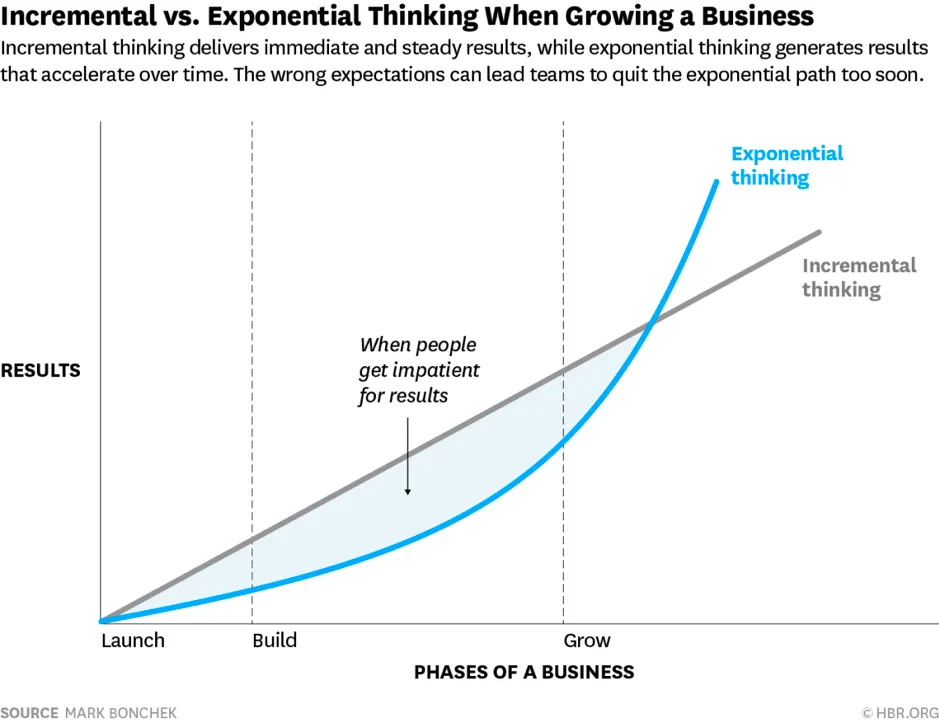
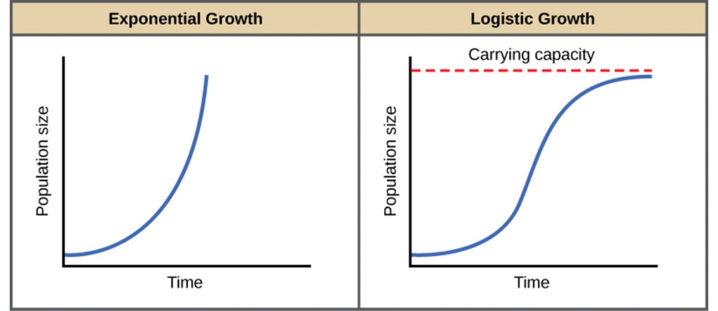
Exponential Models
Used when the rate of change increases based on the current value.
- Example: Population growth or the spread of a viral TikTok video.
Stochastic (Probabilistic) Models
Used when there is randomness involved. Instead of one “right” answer, it gives you a range of probabilities.
- Example: Predicting the weather or stock market fluctuations.
3. Why are they “Always Wrong”?
Statisticians often say, “All models are wrong, but some are useful.” A map of a city is a “model.” If the map were as big and detailed as the actual city, it would be useless. To be useful, a model must leave things out. A mathematical model for a bridge might ignore the color of the paint, but it cannot ignore the wind speed or the weight of the steel.
4. Real-World Applications
- Epidemiology: Predicting how many people will need hospital beds during a flu season.
- Engineering: Testing if a skyscraper can withstand an earthquake before a single brick is laid.
- Climate Science: Using billions of data points to simulate how Earth’s temperature might change over the next century.
How do you make new functions from old functions?
Think of functions like building blocks. Once you have a basic set of “parent” functions—like f(x) = x2 or g(x) = sin(x)—you can combine, stretch, or shift them to create much more complex and useful tools.
Here are the four primary ways to build new functions from old ones.
1. Arithmetic Combinations
Just like regular numbers, you can add, subtract, multiply, or divide functions. If you have two functions, f(x) and g(x), you can create a third function, h(x), using basic math:
- Addition: h(x) = f(x) + g(x)
- Subtraction: h(x) = f(x) – g(x)
- Multiplication: h(x) = f(x) * g(x)
- Division: $h(x) = f(x) / g(x) (as long as g(x) ≠ 0)
Real-world example: If R(x) is the Revenue from selling x items and C(x) is the Cost to make them, the Profit function is P(x) = R(x) – C(x).
2. Transformations (Shifting and Scaling)
You can take an existing function and “tweak” it by adding constants to the input or output. This is how we move graphs around or change their shape.
- Vertical Shift: f(x) + k (Moves the graph up or down).
- Horizontal Shift: f(x – h) (Moves the graph left or right).
- Scaling: a * f(x) (Stretches or compresses the graph vertically).
- Reflection: -f(x) (Flips the graph over the x-axis).
3. Composition (The “Chain” Effect)
This is arguably the most powerful way to make new functions. Instead of adding them together, you put one function inside another.
The notation is (f ∘ g)(x), which means f(g(x)). You take the output of g and use it as the input for f.
The “Coffee” Example:
- Function g: Grinds beans (Input: Beans → Output: Grounds).
- Function f: Brews coffee (Input: Grounds → Output: Coffee).
- Composition f(g(x)): Input: Beans → Output: Coffee.
4. Piecewise Functions
Sometimes one rule isn’t enough. You can create a new function by “gluing” pieces of different functions together based on the input value.
For example, a shipping company might charge a flat rate for light packages but a higher, variable rate for heavy ones:
- If weight w ≥ 5 lbs, cost is $10.
- If weight w > 5 lbs, cost is $10 + 2(w – 5).
Summary Table
| Method | Operation | What it does |
| Arithmetic | f + g or f · g | Combines the values of two functions. |
| Transformation | f(x) + c | Moves or deforms the existing shape. |
| Composition | f(g(x)) | Feeds one function’s output into another. |
| Inverse | f-1(x) | “Undoes” the original function (swaps input and output). |
How do graphing calculators and computers improve function and model representation?
Before graphing calculators and modern software, visualizing a function meant sitting down with a pencil, a ruler, and a table of values to manually plot points. It was slow, prone to human error, and made complex models nearly impossible to “see.”
Today, technology has shifted the focus from the labor of drawing to the logic of the relationship. Here is how they’ve changed the game:
1. Instantaneous Visualization
Computers can calculate thousands of points per second. This allows for high-fidelity representations that reveal “hidden” behaviors of a function, such as sharp turns, asymptotes, or tiny oscillations that a human might miss when plotting by hand.
- Global vs. Local View: You can instantly zoom out to see the “end behavior” of a model (where it goes in the long run) or zoom in to a specific point to see its slope.
2. Dynamic Manipulation (The “What If?” Factor)
One of the most powerful tools in a graphing calculator (like Desmos or Geogebra) is the slider.
Instead of drawing a new graph for y = 2x, y = 3x, and y = 4x, you can create the function y = mx and slide the value of m. This creates a “movie” of the function, showing exactly how changing a single variable stretches, shifts, or flips the model in real-time.
3. Regression and Curve Fitting
Computers excel at inverse modeling. In the past, if you had a cloud of data points, finding the “line of best fit” involved grueling calculus or “eyeballing” it.
Now, you can input a raw data set, and a computer uses algorithms (like Least Squares) to find the exact function that best represents that data.
- Linear Regression: Finding the best straight line.
- Polynomial/Exponential Regression: Finding the best curve.
4. Multi-Dimensional Modeling
Humans struggle to visualize anything beyond three dimensions. Computers can handle multivariate models where dozens of different functions interact.
- 3D Graphing: Computers can render “surfaces” (3D functions) that show how two different inputs affect one output simultaneously.
- Heat Maps: Representing a third or fourth variable using color instead of physical space.
5. Animation and Time-Series
Many real-world models (like weather patterns or engine combustion) aren’t static; they change over time. Computers allow us to add time (t) as a variable, turning a frozen equation into a simulation. This is the bridge between a simple “function” and a working “model.”
Summary: Then vs. Now
| Feature | Manual Graphing | Computer/Calculator |
| Speed | Minutes to hours | Milliseconds |
| Precision | Limited by the tip of the pencil | High-precision floating-point math |
| Experimentation | Difficult (requires erasing/re-drawing) | Instant (sliders and parameters) |
| Data Handling | Only small sets (5–10 points) | Millions of data points (Big Data) |
How does artificial intelligence be used to represent more complicated functions?
When we talk about Artificial Intelligence (AI) representing functions, we are usually talking about Neural Networks. In mathematics, there is a famous concept called the Universal Approximation Theorem. It states that a neural network with even a single “hidden layer” can approximate almost any continuous function, no matter how wiggly or complex it is.+2
Here is how AI handles the “heavy lifting” of complex modeling:
1. The “Lego Block” Approach
AI doesn’t try to find one giant, perfect equation like y = something complicated. Instead, it breaks the problem down into thousands (or billions) of tiny, simple mathematical pieces.
- Linear Parts: Each “neuron” performs a simple weighted sum (like a basic line: y = mx + b).
- Non-Linear Parts: This is the secret sauce. Each neuron passes its result through an Activation Function (like ReLU or Sigmoid). This adds “curves” or “bends” to the math.
By layering these simple parts, the AI builds a massive, multi-dimensional “surface” that can fit incredibly complex data—like recognizing a face in a photo or predicting the next word in a sentence.
2. Learning vs. Designing
In traditional modeling, a human scientist has to guess the shape of the function (e.g., “I think this data looks exponential”).
In AI, the computer discovers the shape:
- Initialization: The AI starts with a random, “wrong” function.
- Backpropagation: It compares its guess to the real data and calculates the error.
- Optimization: It uses Calculus (specifically gradients) to tweak its internal weights, slowly “molding” the function until the error is as small as possible.
3. Handling “High-Dimensional” Space
Traditional functions usually deal with 2 or 3 variables (x, y, z). AI models handle thousands.
- An image is a function where the input is 1,000,000 pixels (variables).
- AI represents this as a function in “high-dimensional space,” finding patterns and correlations that a human could never visualize.
AI vs. Traditional Models
| Feature | Traditional Mathematical Model | AI / Neural Network Model |
| Logic | “Glass Box” (You can see the formula). | “Black Box” (Hard to read the internal math). |
| Flexibility | Rigid; fits specific shapes (lines, curves). | Highly flexible; can fit any shape. |
| Data Needs | Works with small amounts of data. | Requires massive amounts of data. |
| Best For | Understanding why something happens. | Predicting what will happen. |
Why this is a “Revolution”
For decades, we couldn’t write a mathematical function for “What does a cat look like?” because the variables were too complex. AI solved this by proving we don’t need to write the function—we just need to build a system that can learn it.
Would you like to see the specific math behind a Neural Network’s activation function, or perhaps explore a video that visualizes this “Universal Approximation” in action?
Universal Approximation Theorem visual explanation
This video provides a brilliant visual analogy using “Lego blocks” to explain how simple AI components combine to mirror any complex mathematical function.
What are the principles of problem solving?
Problem solving is less about having the “right” answer immediately and more about having a reliable process. Whether you are debugging code, fixing a relationship, or solving a physics equation, most effective methods follow a structured cycle.
The most famous framework was developed by mathematician George Pólya in 1945, and it remains the gold standard today.
1. Understand the Problem
You cannot solve what you don’t define. This stage is about stripping away the noise to find the core issue.
- Identify the Unknown: What exactly are you trying to find or achieve?
- Gather Data: What are the “knowns”? What information do you already have?
- Identify Constraints: What are the “rules”? (e.g., “I need to fix this car, but I only have $50 and two hours.”)
- Restate it: Try explaining the problem to someone else (or a “rubber duck”). If you can’t explain it simply, you don’t understand it yet.
2. Devise a Plan (The Strategy)
This is where you choose your “tools.” There isn’t just one way to solve a problem; instead, you look for a heuristic (a mental shortcut):
- Look for a Pattern: Has something like this happened before?
- Work Backward: Start with the goal and see what the step right before it would be.
- Break it Down: Divide a massive problem into “sub-problems” that are easier to manage.
- Draw a Diagram: Visualizing the relationship between parts often reveals the solution.
3. Carry Out the Plan
This is the execution phase. The key here is patience and precision.
- Step-by-Step: Follow your plan. If it’s a math problem, check each line of your work as you go.
- Persistence: If the plan isn’t working, don’t just give up—identify where it’s failing. Is the plan bad, or is the execution flawed?
- Flexibility: Be prepared to pivot. If your initial strategy hits a dead end, go back to step 2.
4. Look Back (Reflect)
Most people skip this step, but it’s the most important for learning. Once the problem is “solved,” take a moment to evaluate:
- Verification: Does the answer actually make sense? (If you calculated that a trip to the grocery store takes 400 hours, something is wrong).
- Optimization: Is there a simpler way you could have done it?
- Generalization: Can you use this same method to solve other problems in the future?
The “IDEAL” Model
Another popular framework used in business and psychology is the IDEAL cycle:
| Letter | Action | Description |
| I | Identify | Find the problem before it finds you. |
| D | Define | Represent the problem clearly. |
| E | Explore | Look at possible strategies. |
| A | Act | Apply the chosen strategy. |
| L | Look | Evaluate the effects of your action. |
A Pro-Tip: First Principles Thinking
Used by innovators like Elon Musk, this involves “boiling things down to the fundamental truths” and building up from there, rather than reasoning by analogy (doing things just because that’s how they’ve always been done).