What are applications of differentiation?

What is differentiation in a single variable? (Calculus: Fourth Edition

Earth and Atmospheric Sciences

Differentiation is a cornerstone of calculus because it measures how a quantity changes in response to another. In practical terms, it allows us to find the “slope” of a curve at any given point, which translates to finding the rate of change in real-world systems.

Here are the primary applications of differentiation across various fields:

---

1. Optimization (Maxima and Minima)

One of the most common uses of differentiation is finding the highest or lowest point of a function. By setting the first derivative to zero (f'(x) = 0), we can identify critical points where a system is most efficient or profitable.

• Economics: Calculating the maximum profit or minimum cost for manufacturing.
• Engineering: Finding the strongest shape for a structural beam or the most aerodynamic curve for a wing.
• Logistics: Determining the shortest route or the most efficient fuel consumption rate.

2. Physics and Kinematics

In physics, differentiation defines the relationship between displacement, velocity, and acceleration.

• Velocity: The first derivative of displacement with respect to time (v = ds / dt).
• Acceleration: The second derivative of displacement (or the first derivative of velocity) with respect to time (a = dv / dt = d²s / dt²).
• Meteorology: Analyzing pressure gradients to predict wind speeds. A steeper pressure gradient (a higher spatial derivative) indicates stronger winds.

3. Related Rates

Differentiation allows us to find how one variable changes in relation to another when both are changing over time.

• Example: If you are pumping air into a spherical balloon, you can use differentiation to determine how fast the radius is increasing based on the rate at which the volume is increasing.
• Formula: For a sphere, V = (4 / 3)πr³. Differentiating with respect to time t gives: dV / dt = 4πr²dr / dt

4. Tangents and Normals

In geometry and mapping technology, differentiation is used to find the equation of a tangent line to a curve at a specific point.

• Tangent: Represents the instantaneous direction of a curve.
• Normal: The line perpendicular to the tangent, essential in optics (refraction) and calculating forces acting perpendicular to a surface.

5. Stability and Concavity

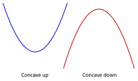
The second derivative ($f”(x)$) tells us about the “shape” of a graph—whether it is concave up (like a cup) or concave down (like a cap).

• Inflection Points: These are points where the concavity changes. In data analysis, this often represents a “diminishing return” or a shift in a trend, such as a change in the spread of a virus or the cooling rate of a substance.

---

Summary Table

Field	Application	Key Derivative Concept
Business	Profit Maximization	First Derivative (f'(x)=0)
Physics	Motion Analysis	Rates of Change (ds / dt, dv / dt)
Chemistry	Reaction Rates	Concentration over time (d[C] / dt)
Biology	Population Growth	Growth rates and carrying capacity

How does differentiation find maximum and minimum values?

To find the maximum and minimum values of a function, we look for points where the function stops increasing and starts decreasing (or vice versa). At these specific “turning points,” the graph of the function is momentarily flat.

In calculus, the derivative represents the slope of the tangent line to a curve. When the slope is zero, the tangent line is horizontal, signaling a potential peak or valley.

---

Example 1:

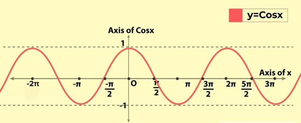
The function f(x) = cos x takes on its (local and absolute) maximum value of 1 infinitely many times, since, since cos 2nπ = 1 for any integer n and -1 ≤ cos x ≤ 1 for all x. Likewise, cos (2n+1)π = -1 is its minimum value, where n is any integer.

Example 2:

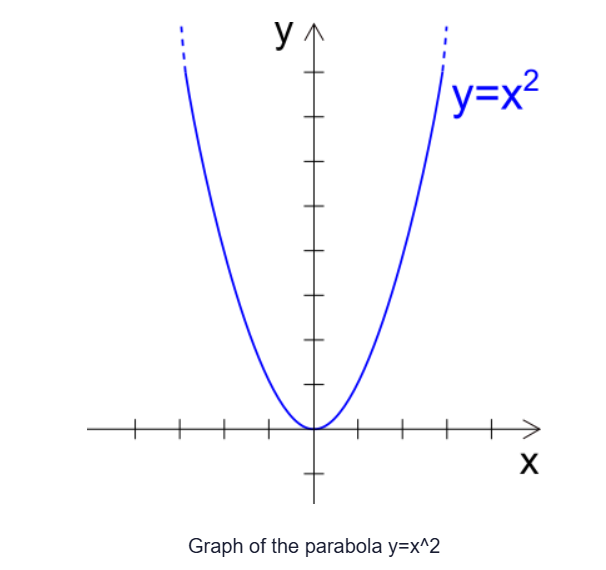
If f(x) = x², then f(x) ≥ f(0) because x² ≥ 0 for all x. Therefore, f(0) = 0 is the absolute (and local) minimum value of f. This corresponds to the fact that the origin is the lowest point on the parabola y = x². However, there is no highest point on the parabola and so this function has no maximum value.

Example 3:

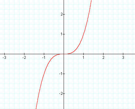
From the graph of the function f(x) = x³ we see that this function has neither an absolute maximum value nor an absolute minimum value. In fact, it has no local extreme values either.

Example 4:

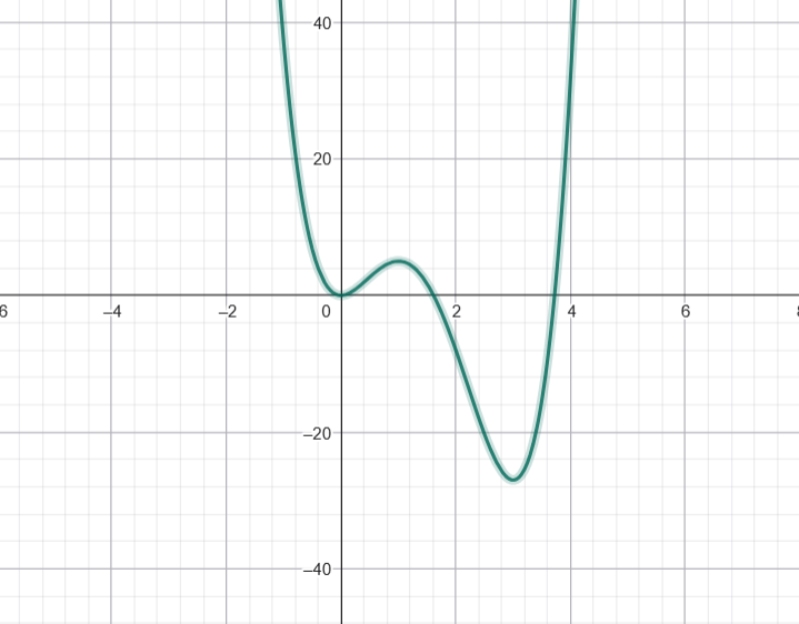
The graph of the function

f(x) = 3x⁴ – 16x³ + 18x² -1 ≤ x ≤ -4 is shown left. You can see that f(1) = 5 is a local maximum, whereas the absolute maximum is f(-1) = 37. [This absolute maximum is not a local maximum because it occurs at an endpoint.] Also, f(0) = 0 is a local minimum and f(3) = -27 is both a local and an absolute minimum. Note that f has neither a local nor an absolute maximum at x = 4.

1. Finding Critical Points

The first step is to calculate the first derivative, f'(x). We then set this derivative to zero and solve for x:

The solutions are called critical points. These are the “candidates” for being a maximum or a minimum because, at these locations, the rate of change is zero.

2. The First Derivative Test

To determine if a critical point is a maximum or a minimum, we look at the behavior of the derivative around that point:

• Local Maximum: If f'(x) changes from positive (climbing) to negative (descending), the point is a peak.
• Local Minimum: If f'(x) changes from negative to positive, the point is a valley.

3. The Second Derivative Test (Concavity)

A faster way to classify these points is to use the second derivative, f”(x), which measures the “bend” or concavity of the curve:

• Local Maximum: If f”(x) < 0, the curve is “concave down” (like an umbrella), meaning the critical point is a maximum.
• Local Minimum: If f”(x) > 0, the curve is “concave up” (like a bowl), meaning the critical point is a minimum.

Example 5:

If f(x) = x³ then f'(x) = 3x², so f'(0) = 0. But f has no maximum or minimum at 0, as shown left. (Or observe that x³ ≥ 0 for x > 0 but x³ < 0 for x < 0). The fact that f'(0) = 0 simply means that the curve y = x³ has a horizontal tangent at (0,0). Instead of having a maximum or minimum at (0,0), the curve crosses its horizontal tangent there.

Example 6:

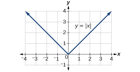
The function f(x) = |x| has its (local and absolute) minimum value at 0, but that value can’t be found by setting f'(x) = 0 because f'(0) does not exist.

Example 7:

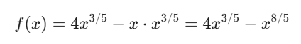
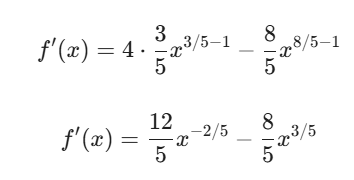
Find the critical numbers of f(x) = x^3/5(4-x).

Solution:

To find the critical numbers of the function f(x) = x^3/5(4-x), we need to determine the values of x in the domain of f where the derivative f'(x) is either zero or undefined.

1. Find the Domain

The function f(x) = x^3/5(4-x) involves a fifth root (x^3/5 = √5(x³)). Since odd roots are defined for all real numbers, the domain of f is (-∞, ∞).

2. Find the Derivative f'(x)

We can find the derivative by first distributing x^3/5:

Now, apply the power rule:

To make it easier to solve, we can factor out the common terms or find a common denominator:

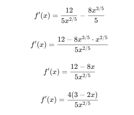
3. Identify Critical Numbers

Critical numbers occur where f'(x) = 0 or where f'(x) is undefined.

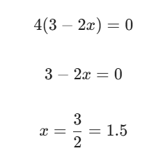
• Where f'(x) = 0:Setting the numerator to zero:

• Where f'(x) is undefined: Setting the denominator to zero:

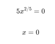
Both x = 0 and x = 1.5 are within the domain of the original function. At x = 1.5, the graph has a horizontal tangent. At x = 0, the derivative is undefined, which typically corresponds to a vertical tangent or a sharp point (cusp).

The critical numbers are x = 0 and x = 3 / 2.

Example 8:

Find the absolute maximum and minimum values of the function

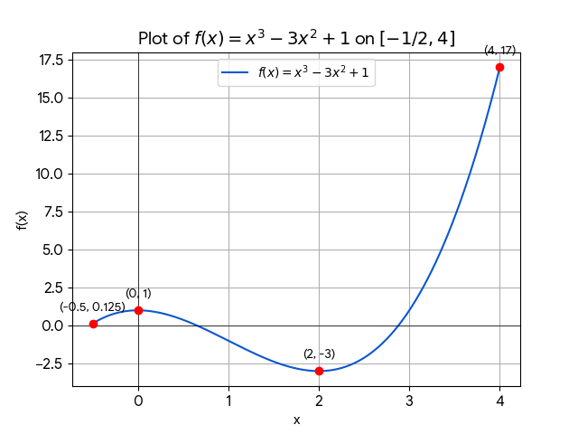
f(x) = x³-3x²+1, -1/2≤x≤4

Solution:

To find the absolute maximum and minimum values of the function f(x) = x³ – 3x² + 1 on the closed interval [-1/2, 4], we follow these steps:

1. Find the Critical Points

First, we find the derivative of the function and set it to zero to locate the critical points.

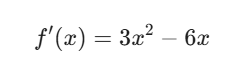
Setting f'(x) = 0:

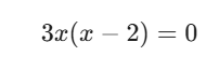
The critical points are x = 0 and x = 2. Both of these points lie within the given interval [-0.5, 4].

2. Evaluate the Function at Critical Points and Endpoints

We evaluate the function at the critical points (x = 0, 2) and the endpoints of the interval (x = -0.5, 4):

• Endpoint x = -0.5: f(-0.5) = (-0.5)³ – 3(-0.5)² + 1 = -0.125 – 0.75 + 1 = 0.125
• Critical Point x = 0: f(0) = (0)³ – 3(0)² + 1 = 1
• Critical Point x = 2: f(2) = (2)³ – 3(2)² + 1 = 8 – 12 + 1 = -3
• Endpoint x = 4: f(4) = (4)³ – 3(4)² + 1 = 64 – 48 + 1 = 17

3. Compare the Values

Comparing the results:

• f(-0.5) = 0.125
• f(0) = 1
• f(2) = -3
• f(4) = 17

The absolute maximum value is 17, occurring at x = 4.

The absolute minimum value is -3, occurring at x = 2.

The plot below visualizes the function over the specified interval, highlighting these points.

---

Real-World Example: Maximizing Revenue

Imagine a business where profit (P) depends on the price (x) of a product. To find the “sweet spot” price that yields the most money:

1. Differentiate the profit function to get P'(x).
2. Set to Zero: Solve P'(x) = 0 to find the optimal price.
3. Verify: Use the second derivative to ensure it’s a maximum (concave down) rather than a minimum.

Why This Matters in Science

In fields like meteorology, this is used to find the center of a high-pressure or low-pressure system. At the exact center of a storm (the minimum pressure), the pressure gradient—or the spatial derivative—is zero, which is often why the “eye” of a storm can have relatively calm winds compared to the surrounding wall.

How does calculus explain rainbows?

Problem 1

Rainbows are created when raindrops scatter sunlight. They have fascinated mankind since ancient times and have inspired attempts at scientific explanation since the time of Aristotle. In this project we use the ideas of Descartes and Newton to explain the shape, location and colours of rainbows.

1. A figure depicts the formation of the primary rainbow showing a ray of sunlight entering a spherical raindrop at a point A. Some of the light is reflected along a line AB, but there’s a part that enters the drop. The light is refracted toward the normal line AO and in fact Snell’s Law says that sin α = k sin β, where α is the angle of incidence, β is the angle of refraction, and k = 4/3 is the index of refraction for water. At B some of the light passes through the drop and is refracted into the air, but the line BC shows the part that is reflected. (The angle of incidence equals the angle of reflection.) What the ray reaches C, part of it is reflected, but for the time being we are more interested in the part that leaves the raindrop at C. (Notice that it is refracted away from the normal line.) The angle of deviation D(α) is the amount of clockwise rotation that the ray has undergone during this three-stage process. Thus D(α) = (α – β) + (π – 2β) + (α – β) = π + 2α- 4β. Show that the minimum value of the deviation is D(α) ≈ 138° and occurs when α ≈ 59.4°.

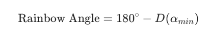
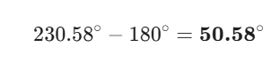
The significance of the minimum deviation is that when α ≈ 59.4° we have D'(α) ≈ 0°, so ΔD / Δα ≈ 0°. This means that many rays with α ≈ 59.4° become deviated by approximately the same amount. It is the concentration of rays coming from near the direction of minimum deviation that creates the brightness of the primary rainbow. The figure shows that the angle of elevation from the observer up to the highest point on the rainbow is 180° – 138° ≈ 42°. (This angle is called the rainbow angle.)

Solution: It is fascinating how Descartes and Newton were able to turn a mystical phenomenon into a predictable mathematical model. To find the minimum deviation, we need to treat the deviation D as a function of the angle of incidence α and find where its derivative is zero.

Step 1: Set up the Derivative

The deviation function is given by:

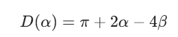
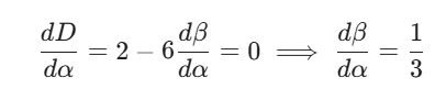
To find the minimum, we differentiate with respect to α:

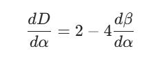
We set this to zero to find the critical point:

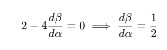
Step 2: Use Snell’s Law

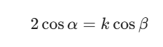
From Snell’s Law, we have sin α = k sin β. Differentiating both sides with respect to α gives:

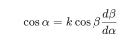
Substituting our value for dβ / dα = 1 / 2:

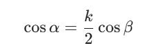
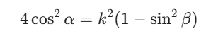
Step 3: Solve for α

To solve for α, we need to eliminate β. We square both sides and use the identity cos²β = 1 – sin²β:

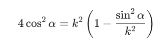
From Snell’s Law, sin²β = sin²α / k². Substituting this in:

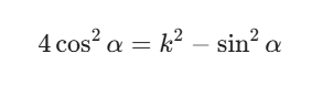
Using sin²α = 1 – cos²α:

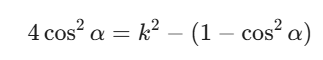
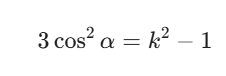
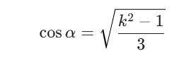
Step 4: Final Calculation

Using k = 4 / 3:

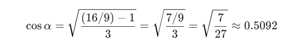
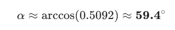
Now, find β using sin β = sin(59.4°) / (4/3) ≈ 0.6455, which gives β ≈ 40.2°.

Plugging these into the deviation formula:

---

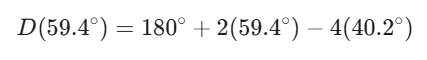
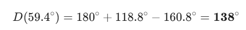
This 138° deviation is the “turning point” for the light rays. Because the change in deviation is so small at this angle, the light “piles up,” creating the intense band of color we see.

Problem 2

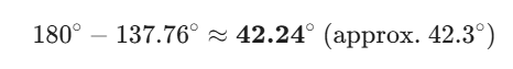
Problem 1 explains the location of the primary rainbow but how do we explain the colours? Sunlight comprises a range of wavelengths, from the red range through orange, yellow, green, blue, indigo, and violet. As Newton discovered in his prism experiments of 1666, the index of refraction is different for each colour. (The effect is called dispersion.) For red light the refractive index is k ≈ 1.3318 whereas for violet light it is k ≈ 1.3435. By repeating the calculation of Problem 1 for these values of k, show that the rainbow angle is about 42.3° for the red bow and 40.6° for the violet bow. So the rainbow really consists of seven individual bows corresponding to the seven colours.

The key to the rainbow’s colors lies in that slight variation in the refractive index, k. Because k is slightly higher for violet light than for red, violet light “bends” more sharply as it enters and leaves the droplet.

To find the rainbow angle (the angle of elevation), we use the formula derived previously:

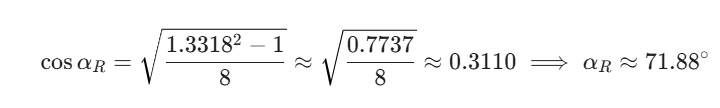
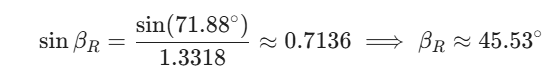
1. Calculation for Red Light (k ≈ 1.3318)

First, find the angle of incidence α that produces the minimum deviation:

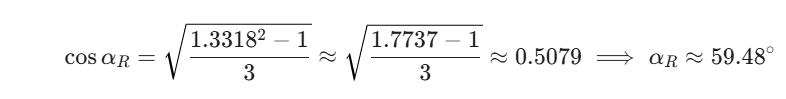
Next, find the angle of refraction β using Snell’s Law (sin β = sin α / k):

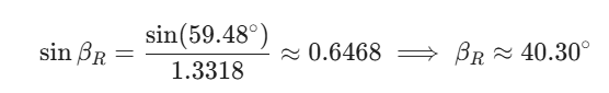
Now, calculate the minimum deviation D(α):

Finally, the rainbow angle is:

---

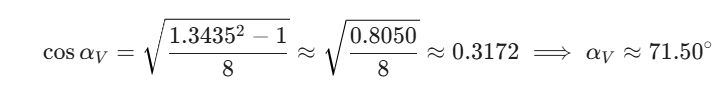
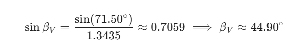
2. Calculation for Violet Light (k ≈ 1.3435)

Repeat the process with the higher refractive index:

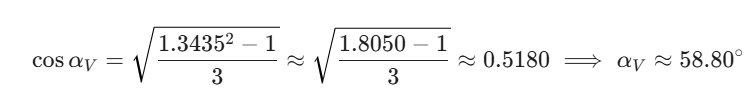
Find β:

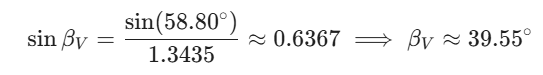
Calculate the minimum deviation:

The rainbow angle is:

Why the Colors Separate

As the calculations show, the “piling up” of light occurs at different angles for different wavelengths. Red light is concentrated at an elevation of roughly 42.3°, while violet light is concentrated lower at 40.6°.

This is why, when you look at a primary rainbow, red is always on the outside (top) of the arc and violet is on the inside (bottom). Each color is essentially its own separate bow, slightly offset from the others due to the physical properties of water and light.

Problem 3

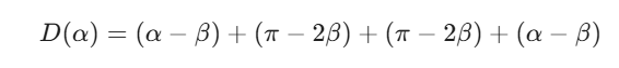
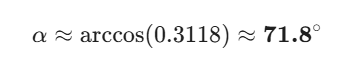
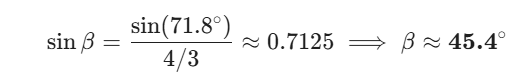
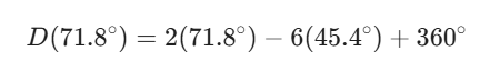
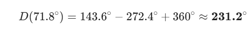
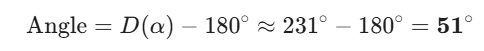
Perhaps you have seen a fainter secondary rainbow above the primary bow. That results from the part of a ray that enters a raindrop and is refracted at A, reflected twice (at B and C), and refracted as it leaves the drop at D. This time the deviation angle D(α) is the total amount of counterclockwise rotation that the ray undergoes in this four-stage process. Show that D(α) = 2α- 6β + 2π and D(α) has a minimum value when cos α ≈ sqrt ((k² – 1)/8). Taking k = 4/3, show that the minimum deviation is about 129° and so the rainbow angle for the secondary rainbow is about 51°.

The secondary rainbow is a beautiful result of light taking a slightly more complex path. In this case, the ray is reflected twice inside the raindrop before it exits, which accounts for its position higher in the sky and why its colors are reversed compared to the primary bow.

Part 1: Deriving the Deviation Function D(α)

For a secondary rainbow, the light undergoes four stages:

1. Refraction at A: Rotation of (α – β)
2. First Reflection at B: Rotation of (π – 2β)
3. Second Reflection at C: Rotation of (π – 2β)
4. Refraction at D: Rotation of (α – β)

Summing these counterclockwise rotations:

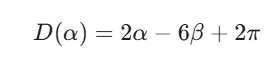
Part 2: Finding the Minimum Deviation

To find the minimum, we differentiate D(α) with respect to α and set it to zero:

Using the derivative of Snell’s Law we established earlier (cos α = k cos β dβ / dα):

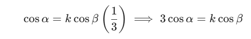
Square both sides to eliminate β:

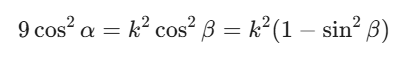
Substitute sin²β = sin²α / k²:

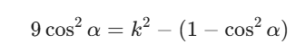
Substitute sin²α = 1 – cos²α:

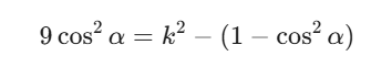
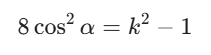
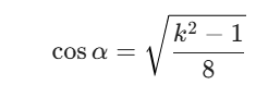
Part 3: Calculating for k = 4/3

Using the index of refraction for water (k ≈ 1.333):

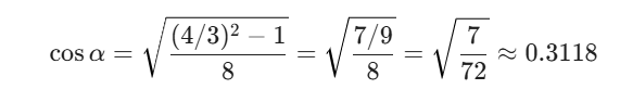
Now, find β:

Plug these into the secondary deviation formula:

The Rainbow Angle

Because the ray has rotated more than 180°, the observer sees the light coming from “behind” the drop relative to the primary ray. The observed angle of elevation (the rainbow angle) is measured from the anti-solar point:

This explains why you always look about 9° higher in the sky to find the secondary bow.

Problem 4

To show why the colors reverse, we apply the secondary rainbow’s deviation formula to the refractive indices for red and violet light. Recall that for the secondary bow, the deviation is $D(\alpha) = 2α – 6β + 2π.

1. Calculation for Red Light (k ≈ 1.3318)

First, find the angle of incidence α for minimum deviation:

Next, find β using sin β = sin α / k:

Calculate the deviation D_R:

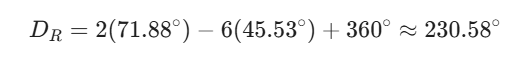
The secondary rainbow angle for red is:

---

2. Calculation for Violet Light (k ≈ 1.3435)

Repeat the steps for the higher refractive index:

Find β:

Calculate the deviation D_V:

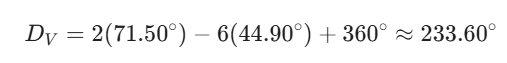
The secondary rainbow angle for violet is:

---

Conclusion: The Reversal

By comparing the elevation angles, we can see the physical “stacking” of the colors in the sky:

Color	Primary Rainbow Angle	Secondary Rainbow Angle
Red	42.3° (Higher)	50.6° (Lower)
Violet	40.6° (Lower)	53.6° (Higher)

In the primary bow, red has the larger angle and appears on the outside of the arc. In the secondary bow, violet has the larger angle (53.6° vs 50.6°), meaning violet is on the outside and red is on the inside.

This inversion happens because the extra internal reflection “flips” the ray paths. Because the secondary bow is formed by two reflections, the light has to travel further and exits at a steeper angle, which also explains why the secondary bow is always fainter—more light is lost with each reflection.

What is the mean value theorem?

The Mean Value Theorem (MVT) is one of the most important theoretical building blocks in calculus. It bridges the gap between the “average” change over an interval and the “instantaneous” change at a specific point.

In simple terms, it states that if you travel from point A to point B, there must be at least one moment during your trip where your instantaneous speed was exactly equal to your average speed.

---

1. The Formal Definition

For a function f(x), the theorem requires two conditions:

1. The function must be continuous on the closed interval [a, b].
2. The function must be differentiable on the open interval (a, b).

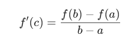
If these hold, then there exists at least one number $c$ in the interval $(a, b)$ such that:

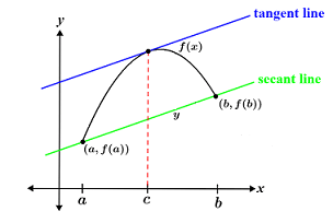
2. Geometric Interpretation

The right side of the equation, (f(b) – f(a)) / (b – a), represents the slope of the secant line connecting the endpoints (a, f(a)) and (b, f(b)).

The left side, $f'(c)$, represents the slope of the tangent line at x = c.

The theorem guarantees that there is a point c where the tangent line is parallel to the secant line.

---

3. Real-World Applications

Speed Traps (Average vs. Instantaneous)

Police often use the MVT for “toll road” speeding tickets. If you enter a highway at 1:00 PM and exit 60 miles away at 2:00 PM, your average speed was 60 mph. Even if a camera never caught you going over 60, the MVT proves that at some specific moment (c) between 1:00 and 2:00, your speedometer (the derivative) read exactly 60 mph. If the speed limit was 50, you were definitely speeding.

Meteorology and Pressure Changes

In atmospheric science, if the barometric pressure drops by 10 hPa over a 5-hour period, the MVT tells us there was at least one instant where the pressure was falling at exactly 2 hPa per hour. This helps in modeling the intensity of developing weather systems.

Physics of Motion

If an object’s position changes over time, the MVT ensures that the object’s instantaneous velocity must have matched its average velocity at some point. This is used to verify consistency in kinematic data.

---

4. Special Case: Rolle’s Theorem

Rolle’s Theorem is a specific version of the MVT. It states that if the starting and ending heights are the same (f(a) = f(b)), then there must be at least one point where the derivative is zero (f'(c) = 0). This is essentially saying that if you end up exactly where you started, you must have stopped or turned around at some point.

How do derivatives affect the shape of a graph?

The shape of a graph is dictated by its derivatives. While the original function f(x) tells you the “where” (the position of a point), the first and second derivatives tell you the “how”—how the graph is moving and how it is bending.

Think of it as a hierarchy of information:

---

1. The First Derivative (f'(x)): Direction

The first derivative measures the slope. It tells you whether the graph is moving up, moving down, or leveling off.

• Increasing: If f'(x) > 0, the graph is climbing from left to right.
• Decreasing: If f'(x) < 0, the graph is falling from left to right.
• Horizontal: If f'(x) = 0, the graph is momentarily flat. This usually indicates a “turning point” like a peak (maximum) or a valley (minimum).

---

2. The Second Derivative (f”(x)): Curvature

The second derivative measures the concavity. It tells you which way the “opening” of the curve faces. It essentially describes the rate at which the slope itself is changing.

• Concave Up: If f”(x) > 0, the slope is increasing. The graph looks like a cup or a smile. It can hold water.
• Concave Down: If f”(x) < 0, the slope is decreasing. The graph looks like a cap or a frown. Water would run off it.
• Inflection Point: If f”(x) = 0 and the sign changes, this is an inflection point. It is where the graph switches from curving one way to the other (like the middle of an “S” curve).

[Image showing concave up and concave down curves with inflection points]

---

3. Summary of Visual Shapes

By combining these two derivatives, we can determine the exact “personality” of any segment of a graph:

f′(x) (Slope)	f′′(x) (Concavity)	Visual Shape	Description
Positive (+)	Positive (+)	⤴	Climbing and getting steeper (accelerating upward).
Positive (+)	Negative (-)	⤵	Climbing but leveling off (slowing down).
Negative (-)	Positive (+)	⤵ (bottom)	Falling but leveling off (approaching a bottom).
Negative (-)	Negative (-)	⤴ (top)	Falling and getting steeper (accelerating downward).

---

Why this matters in Practice

In fields like meteorology, we look at how pressure or temperature changes over distance or time.

• If the temperature is rising (f’ > 0) but the rate of rising is slowing down (f” < 0), we know we are approaching a peak temperature for the day.
• In physics, the first derivative of position is velocity, and the second is acceleration. If the second derivative is positive, you aren’t just moving; you are speeding up.

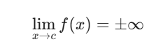
What are limits at infinity and how do they define asymptotes?

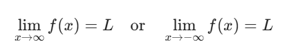
Limits at infinity describe the behavior of a function as the input $x$ becomes extremely large in the positive direction (x → ∞) or extremely large in the negative direction (x → -∞). Essentially, they answer the question: “As we move off the edge of the graph, does the y-value settle down toward a specific number, or does it head off to infinity?”

These limits are the mathematical tools used to define and find asymptotes.

---

1. Horizontal Asymptotes

A horizontal asymptote is a flat line that the graph approaches but often never touches as $x$ goes to infinity.

If the limit of a function as x approaches infinity (or negative infinity) is a finite number L, then the line y = L is a horizontal asymptote.

• Example: For f(x) = 1 / x, as x gets huge, f(x) gets closer to 0. Therefore, y = 0 is the horizontal asymptote.

---

2. Vertical Asymptotes (Infinite Limits)

While horizontal asymptotes look at what happens when x is huge, vertical asymptotes occur when the output f(x) becomes huge as x approaches a specific finite value c.

If the function “blows up” to infinity as you get close to a number c, then the line x = c is a vertical asymptote.

• Example: For f(x) = 1 / (x-2), as x approaches 2, the denominator becomes 0, and the value of the function shoots toward infinity. Thus, x = 2 is a vertical asymptote.

---

3. Slant (Oblique) Asymptotes

A slant asymptote occurs when a function approaches a diagonal line (y = mx + b) as x → ∞. This typically happens in rational functions where the degree of the numerator is exactly one higher than the degree of the denominator.

As x grows, the “fractional” part of the function disappears (goes to 0), leaving only the linear part.

---

Rules of Thumb for Rational Functions

You can often determine horizontal asymptotes just by looking at the highest powers (degrees) of x in a fraction:

Scenario	Resulting Asymptote
Degree of Bottom > Degree of Top	The horizontal asymptote is y = 0.
Degree of Top = Degree of Bottom	The asymptote is the ratio of the leading coefficients.
Degree of Top > Degree of Bottom	There is no horizontal asymptote (it may be a slant asymptote).

Real-World Connection

In meteorology, we often use limits to model how a physical property (like the concentration of a gas or the cooling of a parcel of air) behaves over a very long distance or time. For instance, the “terminal velocity” of a falling raindrop is a horizontal asymptote—it is the speed the drop approaches as time (t) goes to infinity, where the force of gravity is balanced by air resistance.

How can calculus be used to sketch the curve of a graph?

Curve sketching is essentially the process of using calculus to create a highly accurate “skeleton” of a function without needing to plot dozens of individual points. By analyzing the derivatives, you can determine exactly where the graph turns, bends, and levels off.

Here is the systematic “Calculus Toolkit” used to sketch any curve:

---

1. Analyze the Original Function: f(x)

Before using calculus, look at the basic “geography” of the function:

• Domain: Where is the function defined? (Are there values that cause a zero in the denominator?)
• Intercepts: Where does the graph cross the axes?
  • Find the y-intercept by calculating f(0).
  • Find x-intercepts by solving f(x) = 0.
• Asymptotes: Use limits to see how the graph behaves at its boundaries or at infinity.

2. Analyze the First Derivative: f'(x)

The first derivative tells you about the slope and direction.

• Critical Points: Solve f'(x) = 0 to find where the graph is flat (potential peaks or valleys).
• Increasing/Decreasing: Test the intervals between critical points.
  • If f'(x) > 0, the curve is rising.
  • If f'(x) < 0, the curve is falling.
• Local Extrema: Use the First Derivative Test to identify which critical points are Local Maxima (peaks) and Local Minima (valleys).

3. Analyze the Second Derivative: f”(x)

The second derivative tells you about the shape and curvature.

• Concavity: * If f”(x) > 0, the graph is concave up (opening upward like a cup).
  • If f”(x) < 0, the graph is concave down (opening downward like an umbrella).
• Inflection Points: Solve f”(x) = 0 to find where the curve changes its “bend.” This is the point where a graph transitions from concave up to concave down.

---

4. Putting it all Together: The Sketching Process

Once you have these “landmarks,” you can draw the curve with confidence:

1. Plot the points: Mark the intercepts, local maxima, local minima, and inflection points on your grid.
2. Draw the asymptotes: Use dashed lines for vertical or horizontal asymptotes to act as “guide rails.”
3. Connect the dots: Use the concavity and direction info to draw the segments. For example, if a segment is increasing (f’ > 0) but concave down (f” < 0), you draw a curve that rises but begins to level off.

Summary Table for Sketching

If f′(x) is…	And f′′(x) is…	The curve looks like…
Positive (+)	Positive (+)	A steepening climb ⤴
Positive (+)	Negative (-)	A leveling-off climb ⤵
Negative (-)	Positive (+)	A leveling-off descent ⤴
Negative (-)	Negative (-)	A steepening descent ⤵

---

Real-World Application

In meteorology, curve sketching techniques are used to visualize vertical temperature profiles of the atmosphere (soundings). By identifying where the lapse rate (the derivative of temperature with height) changes sign or concavity, meteorologists can identify “inversion layers” where the air becomes very stable, which is crucial for predicting storm development or smog levels.

What is the difference between graphing with calculus and graphing with calculators?

While a graphing calculator provides a fast, high-resolution picture of a function, graphing with calculus provides the mathematical “why” behind the shape. Calculators are excellent for visualization and speed, but they can be misleading; calculus reveals the underlying structure that a screen might miss.

Here is a breakdown of how these two approaches differ in depth, accuracy, and purpose.

---

1. Discovery vs. Documentation

• Graphing with Calculators: A calculator works by “brute force.” it calculates thousands of individual points (x, y) and connects them. It shows you what the graph looks like in a specific window, but it doesn’t “know” what happens outside that window.
• Graphing with Calculus: Calculus identifies the DNA of the curve. By finding derivatives, you find the exact points where the graph must turn (maxima/minima) or change its bend (inflection points). You aren’t just seeing the graph; you are proving its behavior.

2. The “Window” Problem

Calculators can be deceptive if the viewing window is set incorrectly. A graph might look like a straight line on a calculator, but calculus might reveal a hidden peak just outside the screen.

• Calculator Risk: You might miss a vertical asymptote or a sharp turn if it occurs at x = 100 while your screen only goes to x = 10.
• Calculus Advantage: Limits at infinity and the first derivative test will tell you exactly where important features exist, regardless of where you are looking.

3. Precision: Exact vs. Approximate

• Calculators: Most calculators give decimal approximations (e.g., x ≈ 1.414).
• Calculus: Calculus provides exact analytical values (e.g., x = sqrt(2)). In fields like engineering or physics, these exact values are often necessary for further calculations where rounding errors could compound and cause issues.

4. Qualitative vs. Quantitative Analysis

Feature	Graphing Calculator (Quantitative)	Calculus Analysis (Qualitative)
Speed	Instantaneous.	Takes time to derive and solve.
Trend	Shows you the current trend.	Explains the rate of change (acceleration/deceleration).
Concavity	Hard to see exactly where a curve flips.	The second derivative (f”) pinpoints the inflection point.
Asymptotes	May show a “connector” line that isn’t real.	Defines the exact boundary lines (y=L or x=c).

---

Real-World Integration

In professional fields like meteorology or data science, these two methods are used together. An IT specialist or meteorologist might use a computer model (the “calculator”) to generate a forecast graph, but they use calculus to verify the stability of the model. If the computer shows a sudden spike in pressure, the scientist uses the derivatives to determine if that spike is a physical reality or just a mathematical error in the software.

Summary

Graphing with a calculator is like looking at a photograph: it’s a great snapshot of a moment. Graphing with calculus is like looking at a blueprint: it explains how the structure was built and exactly how it will behave under any condition.

What are optimization problems?

Optimization problems are mathematical challenges where the goal is to find the best possible solution from a set of available choices. In calculus, “best” typically means either maximizing something desirable (like area, profit, or efficiency) or minimizing something undesirable (like cost, time, or waste).

At its core, an optimization problem asks: What value of x will give me the largest or smallest value of y?

---

1. The Anatomy of an Optimization Problem

Every optimization problem consists of two main components:

• The Objective Function: This is the primary equation representing the quantity you want to optimize (e.g., V for volume or C for cost).
• The Constraint: These are the real-world limitations (e.g., you only have 100 meters of fencing, or a budget of 500). Constraints allow you to reduce the problem to a single variable so you can differentiate it.

---

2. How Calculus Solves Them

Optimization relies on the fact that the maximum or minimum of a smooth function occurs at a critical point—where the derivative is zero.

The Standard Procedure:

1. Identify the variables and what needs to be optimized.
2. Write the Objective Function (e.g., Area = length * width).
3. Use the Constraint to substitute variables until the function has only one independent variable.
4. Differentiate the function and set the derivative to zero (f'(x) = 0).
5. Solve for x and verify it’s a max or min using the Second Derivative Test.

---

3. Classic Examples

The “Fencing” Problem (Geometry)

A farmer has 200 meters of fencing and wants to enclose a rectangular field next to a straight river (so no fencing is needed on the river side). What dimensions provide the maximum area?

• Constraint: 2w + l = 200
• Objective: Area = w * l
• By substituting l = 200 – 2w into the area formula, you get a parabola. Finding the vertex (where the derivative is zero) gives the optimal width.

The “Open Box” Problem (Manufacturing)

If you have a square sheet of cardboard and cut equal squares out of the corners to fold it into a box, how large should the cuts be to maximize the volume?

Least Time (Physics/Optics)

Light travels between two points by the path that takes the least time. This is known as Fermat’s Principle. Calculus is used to prove that the “path of least time” is why light bends when it moves from air to water (Snell’s Law).

---

4. Professional Applications

• Meteorology: Models use optimization to find the “best fit” for data points when initializing a weather forecast. This minimizes the error between observed weather and the starting state of the simulation.
• Information Technology: Optimization algorithms are used to route data packets through a network via the path with the lowest latency (minimum time).
• Logistics: Companies like FedEx or UPS use these principles to minimize fuel consumption by optimizing delivery routes.

---

Summary Table: Maximize vs. Minimize

Goal	Common Metric	Calculus Condition
Maximize	Profit, Area, Volume, Efficiency	f'(x)=0 and f”(x) < 0 (Concave Down)
Minimize	Cost, Distance, Time, Waste	f'(x)=0 and f”(x) > 0 (Concave Up)

How does calculus explain the shape of cans in a grocery store?

The shape of a standard aluminum can is a classic example of an optimization problem in calculus. Manufacturers want to minimize the cost of materials while maximizing the amount of product inside.

Since the cost of a can is primarily determined by the amount of metal used (surface area), the goal is to find the dimensions of a cylinder that minimize surface area for a fixed volume.

---

1. The Mathematical Setup

To solve this, we define the two primary equations for a cylinder (the can):

• Objective Function (Surface Area): The total metal used for the top, bottom, and the curved side.A = 2πr² + 2πrh
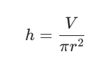
• Constraint (Volume): The amount of liquid the can must hold (e.g., 355 mL). V = πr²h

2. Reducing the Variables

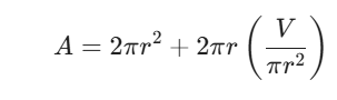
To use differentiation, we need the surface area equation to have only one variable. We use the volume constraint to solve for h:

Now, substitute this h into the Surface Area formula:

---

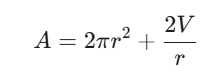
3. Finding the Minimum (Differentiation)

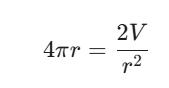
To find the radius (r) that uses the least amount of metal, we take the derivative of the area with respect to r and set it to zero:

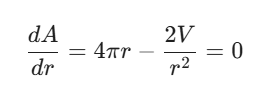
Solving for V:

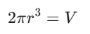
Since we know V = πr²h, we can substitute it back:

Dividing both sides by πr² gives:

h = 2r (or h = d, the diameter)

---

4. Why aren’t all cans perfect squares?

Calculus suggests the most efficient can is one where the height is equal to the diameter. This would look like a “square” profile from the side. However, if you look at a shelf in a grocery store, many cans (like soda cans) are taller and thinner. Why?

• Human Factors: A slightly taller, thinner can is easier for a human hand to grip comfortably.
• Structural Integrity: The top and bottom of a can are often thicker than the sides to withstand the pressure of carbonation. Calculus can be adjusted to account for “weighted” costs where the ends cost more than the sides, leading to a taller shape.
• Marketing & Shelving: Taller cans can sometimes appear “larger” to consumers and allow for more units to be packed side-by-side on a narrow shelf.

Summary

Calculus provides the “ideal” starting point for industrial design. By finding the derivative of the material cost function, engineers can determine exactly how much they are “paying” in extra aluminum to make a can more ergonomic or visually appealing.

What are applications of differentiation to economics?

In economics, differentiation is the primary tool used for marginal analysis. Since economics often focuses on how a small change in one variable (like price or production) affects another (like profit or demand), the derivative provides the exact “rate of change” necessary for decision-making.

Here is how differentiation drives economic theory and practice:

---

1. Marginal Functions

The term “marginal” in economics is synonymous with the “derivative” in calculus. It represents the additional cost or revenue generated by producing one more unit.

• Marginal Cost (MC): The derivative of the total cost function C(x) with respect to the quantity (x). MC = dC / dx
• Marginal Revenue (MR): The derivative of the total revenue function R(x). MR = dR / dx
• Marginal Profit (MP): The derivative of the total profit function (P(x)).

Understanding these rates helps businesses determine if increasing production will actually add to the bottom line or if the cost of that “extra” unit exceeds the revenue it brings in.

2. Profit Maximization

One of the most fundamental rules in economics is that profit is maximized when Marginal Revenue equals Marginal Cost (MR = MC).

Using the rules of optimization:

1. Define the Profit function: P(x) = R(x) – C(x).
2. Find the derivative: P'(x) = R'(x) – C'(x).
3. Set the derivative to zero: 0 = R'(x) – C'(x), which simplifies to R'(x) = C'(x).

3. Price Elasticity of Demand

Differentiation is used to calculate elasticity, which measures how sensitive consumers are to price changes. It is defined as the percentage change in quantity demanded divided by the percentage change in price.

The formula for point elasticity (E_d) uses the derivative of the demand function (Q):

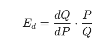
• If |E_d| > 1, the product is elastic (luxury goods; price changes significantly affect demand).
• If |E_d| < 1, the product is inelastic (necessities like fuel or medicine; demand stays relatively stable regardless of price).

4. Minimizing Average Cost

Businesses often want to find the “efficient scale” of production—the point where the cost per unit is as low as possible.

• Average Cost (AC): AC = C(x) / x.
• By taking the derivative d / dx (C(x) / x) and setting it to zero, an economist can find the exact production volume that minimizes the unit cost.

---

5. Inventory and Logistics (EOQ Model)

The Economic Order Quantity (EOQ) model uses differentiation to minimize the total cost of inventory. There is a “tug-of-war” between two costs:

1. Ordering Costs: High if you order small amounts frequently.
2. Holding Costs: High if you order a massive amount and have to store it.

By differentiating the total cost function (Ordering + Holding) and solving for zero, calculus provides the “ideal” order size that balances these two competing expenses perfectly.

---

Summary of Economic Derivatives

Economic Term	Calculus Equivalent	Business Question Answered
Marginal Cost	C'(x)	“How much does the next unit cost to make?”
Marginal Revenue	R'(x)	“How much will I earn from the next sale?”
Optimization	P'(x) = 0	“How many units should I sell to make the most money?”
Elasticity	(dQ / dP) • (P / Q)	“Can I raise prices without losing all my customers?”

What is Newton’s method?

Newton’s Method (also known as the Newton-Raphson method) is a powerful numerical technique used to find the roots of a function—the values of x where f(x) = 0.

While some equations (like quadratics) can be solved with a formula, many complex functions are impossible to solve algebraically. Newton’s Method uses differentiation to “zoom in” on the answer through a series of increasingly accurate guesses.

---

1. The Core Concept: Linear Approximation

The logic behind the method is that if you are close to a root, the tangent line at your current guess is a good approximation of the function itself.

1. You start with an initial guess, x₀.
2. You find the tangent line at that point.
3. Where that tangent line crosses the x-axis becomes your next, better guess (x₁).
4. You repeat the process until the value stabilizes.

2. The Formula

The formula for the (n+1)-th guess is derived from the slope of the tangent line (m = f'(x_n)):

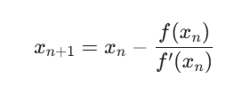
This equation essentially says: “Take your current position and subtract a correction factor based on how high the function is (f(x_n)) and how steep the slope is (f'(x_n)).”

---

3. Step-by-Step Example: Finding sqrt(2)

Finding sqrt(2) is the same as finding the root of f(x) = x² – 2.

• The Derivative: f'(x) = 2x.
• Initial Guess: Let’s guess x₀ = 1.5.
• First Iteration:

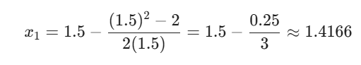
• Second Iteration: Using x₁ in the same formula gives x₂ ≈ 1.4142.

In just two steps, we’ve reached a value that is accurate to four decimal places.

---

4. When Newton’s Method Fails

Because the method relies on the derivative, there are specific “traps” that can cause it to fail:

• Horizontal Tangents: If f'(x_n) = 0, the formula involves dividing by zero. Geometrically, a horizontal tangent line never crosses the x-axis.
• Cycles or Divergence: If your initial guess is poor, the method might bounce back and forth between two values or shoot off toward infinity.
• Multiple Roots: If a function has several roots, the one the method finds depends entirely on where your initial guess starts.

[Image showing Newton’s Method failing due to a horizontal tangent or a starting point far from the root]

---

5. Professional Applications

• Computer Science & IT: Newton’s method is built into the back-end of many software programs (like Excel’s “Goal Seek” or optimization libraries) to solve non-linear equations quickly.
• Meteorology: When running atmospheric models, scientists often have to solve systems of “primitive equations” that don’t have exact solutions. Iterative methods like this one allow computers to approximate pressure and wind fields.
• Physics: Finding the equilibrium points in complex gravitational or electromagnetic fields often requires numerical root-finding.

What are antiderivatives?

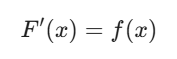
In calculus, an antiderivative is the inverse operation of a derivative. If differentiation tells you the rate at which a quantity is changing (the “slope”), antidifferentiation allows you to work backward from that rate of change to find the original quantity.

Mathematically, a function F is an antiderivative of f if the derivative of F is equal to f:

---

1. The Concept of “Reversing” Change

Think of the relationship between position, velocity, and acceleration.

• If you have your position, you differentiate to find velocity.
• If you have your velocity, you find the antiderivative to recover your position.

2. The Constant of Integration (+ C)

One unique aspect of antiderivatives is that they are not unique. Because the derivative of any constant (like 5, 10, or π) is zero, multiple functions can have the exact same derivative.

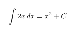
For example, if f(x) = 2x, the antiderivative could be:

• x² (because d / dx (x²) = 2x
• x² + 5 (because d / dx (x² + 5) = 2x
• x² – 100 (because d / dx (x² – 100) = 2x

To account for this, we always add a constant of integration, denoted as + C. The family of all antiderivatives for 2x is written as:

3. Notation: The Indefinite Integral

The process of finding an antiderivative is called integration. We use the integral symbol ∫ to denote this:

• f(x): The integrand (the rate of change).
• dx: The variable we are integrating with respect to.
• F(x) + C: The general antiderivative.

---

4. Why Antiderivatives Matter

Antiderivatives are the key to the Fundamental Theorem of Calculus, which links the slope of a curve to the area underneath it.

Applications:

• Physics: If you know the acceleration of a falling object (like a raindrop), you can integrate it once to find its velocity and a second time to find its exact height at any moment.
• Economics: If you know the marginal cost of producing items (the cost of the “next” item), you can find the antiderivative to determine the total cost of production.
• Engineering: Antiderivatives are used to calculate the accumulation of stress, energy, or fluid flow over time.

---

Summary Table: Derivative vs. Antiderivative

Concept	Direction	Physical Meaning
Derivative	Forward (f → f’)	Instantaneous rate of change (Slope).
Antiderivative	Backward (f’ → f)	Total accumulation or original state.

Solved Problems

What is differentiation in a single variable? (Calculus: Fourth Edition

Earth and Atmospheric Sciences