What problems can calculus solve?

Calculus I – Differentiation of a Single Variable

What problems can calculus solve?

Before calculus was invented, mathematics was primarily “static”—it was great for measuring shapes that didn’t move (like triangles or circles) or calculating fixed values.

Calculus was developed to measure a dynamic universe. At its core, calculus is the mathematics of change and motion (Tarasov, 2019). It allows us to take things that are continuously changing—like the speed of a falling object, the growth of a population, or the flow of electricity—and analyze them precisely (Tarasov, 2019).

Calculus breaks down these complex, changing systems into two fundamental types of problems: Differential Calculus (finding the rate of change) and Integral Calculus (finding the accumulation of a quantity) (Tarasov, 2019).

The Rate of Change Problem (Differential Calculus)

In algebra, you learn how to find the slope of a straight line. But what happens if you want to find the slope of a curve, or the exact speed of an accelerating car at one single, instantaneous moment?

Algebra cannot solve this because finding a slope requires two points (change in y/change in x). If you only look at one single instant, the change in time is zero, and you cannot divide by zero.

The Solution: Differential calculus introduces the concept of a derivative. By using “limits,” it allows us to look at an interval of time so infinitely small that it effectively gives us the instantaneous rate of change—the exact slope of a curve at a single point.

Real-World Applications:

• Physics & Motion: Calculating instantaneous velocity and acceleration. If you know a rocket’s position function, the derivative tells you its exact speed at second 4.
• Optimization: Finding the maximum or minimum of a curve. Businesses use derivatives to find the exact production level that will maximize profit or minimize cost. Engineers use it to find the maximum weight a bridge can hold using the minimum amount of material.

The Accumulation & Area Problem (Integral Calculus)

Geometry makes it easy to find the area of a rectangle (A = l × w) or a triangle

But how do you calculate the exact area under a wavy, unpredictable curve, or the volume of an irregularly shaped object like a flower vase or a human heart?

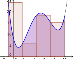
The Solution: Integral calculus introduces the integral. Imagine filling the area under a curve with narrow vertical rectangles. If you use 5 rectangles, your area estimate is rough. If you use 100, it gets much closer. If you use an infinite number of infinitely thin rectangles, you get the exact area. Integration accumulates all these tiny pieces back into a whole.

Real-World Applications:

• Engineering: Finding the center of mass of an oddly shaped airplane wing, or calculating the total structural load on a curved dam.
• Medicine: Measuring cardiac output. Doctors inject a dye into the bloodstream and use integration to calculate the area under the dye-concentration curve, which reveals how efficiently the heart is pumping blood.
• Environmental Science: Calculating the total amount of a pollutant that has leaked into a river over a period of hours when the flow rate was constantly fluctuating.

Predicting the Future (Differential Equations)

Often in real life, we don’t know the exact formula for how a population grows, but we do know the rules governing how it changes. For instance, we know a population’s growth rate is directly proportional to its current size (more people = more babies).

A differential equation is an equation that contains derivatives (rates of change). Solving these equations allows us to turn a known rate of change into a predictive formula for the future.

Real-World Applications:

• Epidemiology: Predicting how fast a virus will spread through a city so hospitals can prepare.
• Space Travel: Plotting the trajectory of a spacecraft. Because planets are constantly moving and pulling on the spacecraft with changing gravitational force, NASA must use systems of differential equations to navigate.
• Economics: Modeling market trends, inflation, and the way consumer demand shifts when prices change (Tarasov, 2019).

Summary Checklist for Students

Whenever you look at a problem, ask yourself:

1. Am I trying to find how fast something is changing right now? → Use a Derivative (Differential Calculus).
2. Am I trying to add up a bunch of continuously changing pieces to find a total? → Use an Integral (Integral Calculus).

References

Tarasov, V. (2019). On history of mathematical economics: Application of fractional calculus. Mathematics, 7(6), 509. https://doi.org/10.3390/math7060509

What is the area problem?

The Area Problem is one of the classic foundational problems that led to the invention of calculus.

Simply put, the problem is this: How do you find the exact area of a shape with curved, irregular borders?

While basic geometry gives us neat formulas for straight-sided shapes, it fails when shapes begin to curve or change dynamically. Calculus solves this by turning the problem into an infinite game of approximation.

Why Geometry Fails

If you need to find the area of a floor to lay down carpet, and the room is a perfect rectangle, geometry makes it easy: Area=length×width. If the room is a triangle or a circle, you have reliable formulas like A=21​bh or A=πr2.

But imagine you are a civil engineer designing a concrete dam, or an environmental scientist tracking a toxic spill along a winding riverbank. The shape under the curve isn’t a perfect circle or a rectangle—it is completely irregular.

Geometry doesn’t have a formula for a shape with a wavy top. This roadblock is exactly what the Area Problem addresses.

The Calculus Solution: Riemann Sums

Calculus solves the Area Problem using a brilliant strategy: break a hard problem down into an infinite number of easy problems. This method is known as finding a Riemann Sum, named after the mathematician Bernhard Riemann.

Here is how it works step-by-step:

The Rough Approximation (A Few Large Rectangles)

We might not know the formula for a curve, but we definitely know the formula for a rectangle. To estimate the area under a curve, we can fill the space with a few vertical rectangles.

• The width of each rectangle is a set interval along the bottom axis (Δx).
• The height of each rectangle is determined by where it touches the curve (f(x)).

If we only use 4 or 5 wide rectangles, our calculation is incredibly fast, but it’s inaccurate. The tops of the rectangles will either stick out past the curve (overestimating the area) or leave empty gaps beneath it (underestimating the area).

Improving Accuracy (More, Thinner Rectangles)

To get a better estimate, we slice the area into more rectangles that are much thinner.

• If we use 20 rectangles instead of 4, the gaps and overlaps become significantly smaller.
• If we use 100 rectangles, the jagged tops of the rectangles begin to closely mimic the smooth slope of the curve. The error shrinks dramatically.

The Perfect Answer (The Definite Integral)

This is where the magic of calculus happens. What if we don’t just use 100 or 1,000 rectangles? What if we use an infinite number of infinitely thin rectangles?

By applying the concept of a limit, calculus allows us to find what value the total area approaches as the width of our rectangles shrinks toward zero. This process is called integration.

The notation looks like this:

• The ∫ symbol is an elongated “S”, which stands for “summation” (adding everything up).
• f(x) represents the height of each infinitely thin slice.
• dx represents the infinitely small width of each slice.

When you compute a definite integral, you are adding up an infinite number of microscopic rectangular areas to find the absolute, exact area under that curve.

Why Does the Area Problem Matter?

Solving the Area Problem isn’t just an abstract exercise for math class; it is how we calculate cumulative totals in the real world when rates are constantly changing.

• Distance Traveled: If an object moves at a constant speed, Distance=Speed×Time (just like a basic rectangle). But if a rocket is accelerating and its speed changes every millisecond, graphing its speed over time creates a curve. The area under that curve equals the exact total distance the rocket traveled.
• Structural Engineering: When building curved architectural arches or boat hulls, calculating the exact surface area and volume is vital to knowing how much material to buy and how much weight the structure can safely support.
• Energy Consumption: If you graph a city’s electricity usage over a 24-hour period, the demand spikes in the afternoon and drops at night. Integrating the area under that fluctuating curve tells power companies exactly how many total megawatt-hours of electricity were consumed that day.

What is the tangent problem?

The Tangent Problem is the second foundational puzzle that sparked the creation of calculus. It is the geometric twin to the Area Problem.

While the Area Problem looks at accumulation, the Tangent Problem looks at direction and speed. Simply put: How do you find the exact slope of a straight line that touches a curve at only one single point?

To understand why this is a problem, we have to look at where traditional algebra stops working.

The Boundary of Algebra: Secant vs. Tangent

In algebra, finding the slope of a line is straightforward. Slope represents the steepness or the rate of change, calculated as:

Notice that this formula requires two points.

• A Secant Line: If you pick two distinct points on a curve and draw a straight line through them, you have a secant line. Because you have two points, algebra easily calculates the slope. This tells you the average rate of change between those two places.
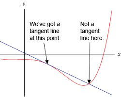
• A Tangent Line: A tangent line is a straight line that skims past a curve, touching it at exactly one unique point, matching the curve’s direction at that precise spot. This represents the instantaneous rate of change.

If you try to use the classic algebra formula to find the slope of a tangent line, you run into a mathematical wall. Because there is only one point, x₁ is equal to x₂. Your formula becomes:

Division by zero is undefined. Algebra cannot calculate how steep a curve is at an absolute, frozen instant in time.

The Calculus Solution: Zooming In with Limits

Calculus solves the Tangent Problem using Differential Calculus and the concept of a limit. Instead of trying to calculate the single point directly, we use a secant line to sneak up on it.

Step 1: Start with an Average

Imagine you want to find the exact slope of a curve at a single target point, P. You start by picking a second point, Q, somewhere further down the curve. You draw a secant line through P and Q and calculate its slope. This gives you a rough approximation of the slope at point P, but it’s not perfect because the curve bends between the two points.

Step 2: Slide the Points Together

Now, imagine sliding point Q down the curve, moving it closer and closer to your target point P. As the distance between the two points shrinks, the secant line rotates.

• If Q is 1 unit away, the slope is a decent guess.
• If Q is 0.1 units away, the slope is incredibly close.
• If Q is 0.00001 units away, the line passing through them is virtually indistinguishable from the true tangent line.

Step 3: Apply the Limit (The Derivative)

Calculus asks: As the distance between P and Q approaches zero, what value does the slope approach? By calculating this limit, we find the exact slope of the tangent line at point P. This resulting value is called the derivative. It allows us to calculate the exact slope of a changing curve anywhere we want.

Why the Tangent Problem Matters in the Real World

Solving the Tangent Problem fundamentally changed how we study physics, engineering, and economics because slope represents a rate of change.

• Instantaneous Velocity: Imagine you are driving a car. If you travel 100 kilometers in 2 hours, your average speed was 50 km/h (this is a secant line calculation). But if you look down at your speedometer at exactly 1 hour and 15 minutes, it might say 72 km/h. That speedometer reading is the instantaneous rate of change—the slope of the tangent line on a graph of your position over time.
• Rocketry and Trajectories: When a spacecraft or an aircraft turns, its momentum at any given fraction of a second is directed along the tangent line of its flight path. Engineers must calculate these tangents to program autopilot systems, thruster burns, and emergency escape vectors.
• Machine Learning and AI: Modern artificial intelligence models learn through a process called “gradient descent.” The AI looks at its current error rate on a multi-dimensional curve and uses derivatives (slopes of tangent lines) to figure out exactly which direction to tweak its parameters to minimize mistakes and optimize performance.

What is velocity?

In physics, velocity is the rate at which an object changes its position in a specific direction.

People often use the words “speed” and “velocity” interchangeably in everyday conversation, but in science, they mean two very different things. The key difference comes down to a single factor: direction.

Speed vs. Velocity: What’s the Difference?

To understand velocity, it helps to compare it directly to speed. In physics, quantities are divided into two categories: scalars (which only have a magnitude/size) and vectors (which have both a magnitude and a specific direction).

• Speed is a scalar quantity. It tells you how fast an object is moving, but it doesn’t care where it’s going. For example: “The airplane is traveling at 800 km/h.”
• Velocity is a vector quantity. It tells you how fast an object is moving and the exact direction it is traveling. For example: “The airplane is traveling at 800 km/h due North-West.”

Because direction matters, two objects can have the exact same speed but completely different velocities. If one car drives east at 60 km/h and another drives west at 60 km/h, their speeds are identical, but their velocities are opposite.

Average Velocity vs. Instantaneous Velocity

Just like calculus splits lines into averages and exact moments, physics splits velocity into two types:

Average Velocity

Average velocity looks at the big picture over a specific window of time. It is calculated by taking an object’s total displacement (the straight-line distance from the starting point to the ending point) and dividing it by the total time it took.

The Track Trap: Imagine a runner completes a perfect 400-meter circular track lap in 60 seconds. Because they started and stopped in the exact same spot, their total displacement is zero. Therefore, even though their average speed was high, their average velocity for that lap is exactly zero!

Instantaneous Velocity

Instantaneous velocity is how fast and in what direction an object is moving at one exact, frozen millisecond. This is where the Tangent Problem from calculus comes into play.

If you graph an object’s changing position over time, the average velocity is represented by a straight secant line connecting two points. To find the instantaneous velocity at a single second, you must calculate the derivative—the slope of the tangent line touching that exact point on the curve.

Velocity in Real-World Motion

Understanding velocity as a vector is essential for navigating a dynamic universe:

• Subway and Transit Systems: A train might maintain a steady speed of 50 km/h to keep passengers comfortable, but every time it rounds a bend or changes tracks, its velocity changes because its direction is altering.
• Spacecraft Navigation: When navigating a vessel or satellite through orbit, engineers cannot just track speed. They must calculate three-dimensional velocity vectors to ensure the spacecraft hits its precise orbital insertion window rather than drifting off into deep space.
• Vector Mechanics in Game Design: When programming objects moving across a screen—like an aircraft dodging obstacles or firing projectiles—developers use separate velocity components for the horizontal movement (v_x) and vertical movement (v_y). Combining these components determines the true speed and angle of the object.

What is the limit of a sequence?

The limit of a sequence is a foundational concept in mathematics that describes the long-term behavior of an ordered list of numbers.

Essentially, it answers the question: As you move further and further down an infinite list of numbers, do the terms get closer and closer to a single, specific value?

If the numbers stabilize around a unique target value, we say the sequence converges to that limit. If they do not, the sequence diverges.

Understanding by Example

A sequence is just a list of numbers following a specific rule, written as $a_1, a_2, a_3, \dots, a_n$. Let’s look at three different types of behavior to see how limits work.

Example 1: The Shrinking Fractions (Convergence)

Consider the sequence where each term is given by the formula a_n = 1/n:

As you look further down the list (as n gets massive), the numbers become microscopic fractions. They will never actually reach absolute zero, but they get infinitesimally close to it.

Because we can get as close to 0 as we want simply by traveling far enough out in the sequence, we say the limit of this sequence is 0.

Mathematically, we write this using limit notation:

(Read as: “The limit as n approaches infinity of 1 over n equals 0.”)

Example 2: The Rocket (Divergence to Infinity)

Now look at a sequence that just keeps growing, like a_n = 2n:

As n goes to infinity, the terms grow without bound. Because these numbers do not settle down or stabilize around a single fixed value, this sequence does not have a finite limit (we say it diverges to infinity).

Example 3: The Ping-Pong Ball (Divergence by Oscillation)

Consider the sequence a_n = (-1)ⁿ:

Even if you travel a billion terms out, the sequence is still bouncing back and forth between -1 and +1. It never settles down on a single number. Because it fluctuates forever, the limit does not exist.

The Formal Definition: The ε-N Game

To turn this intuitive idea into a rigorous mathematical tool, mathematicians use what is famously called the formal definition of a limit.

A sequence a_n converges to a limit L if, for every tiny positive number ε (epsilon), there exists a starting point N such that all terms after N are within a distance of ε from L.

Think of this like a game of target practice:

1. The Challenger picks a target boundary around the limit L, called L ± ε. No matter how tiny or strict they make this error margin ε (e.g., within 0.00001), the rule must hold.
2. The Mathematician wins if they can look down the sequence and find a specific cutoff index, N. Every single number in the list past that cutoff point (n > N) must land perfectly inside the challenger’s tiny boundary.

If the numbers permanently trap themselves inside that boundary, no matter how narrow the challenger makes it, the limit is officially proven to be L.

Why Sequence Limits Matter

Sequence limits are the building blocks for the rest of calculus:

• Defining Functions and Curves: Continuous functions can be analyzed by looking at sequences of discrete points that get infinitely closer together.
• Infinite Series: If you want to add up an infinite list of numbers (like 1/2 + 1/4 + 1/8 + …), you do it by turning the running tallies into a sequence of partial sums. Finding the limit of that sequence tells you the exact sum of the infinite series.
• Computer Simulations: When a computer calculates complex values like π, square roots, or physics trajectories, it often uses iterative algorithms. Each iteration generates a new number in a sequence. Understanding the limit ensures the programmer knows the computer’s answer is actually narrowing in on the correct mathematical truth.

What is a series and is it possible to find its sum?

In mathematics, a series is what you get when you take a sequence of numbers and add them all together.

While a sequence is just an ordered list of separate items, a series is the continuous accumulation of those items. It is often written using the Greek capital letter Sigma (∑), which stands for “summation.”

Is It Possible to Find the Sum of an Infinite Series?

Intuitively, your brain might say: “If you keep adding positive numbers together forever, the total must eventually blow up to infinity.” Surprisingly, the answer is yes—you can find the exact, finite sum of an infinite series, but only under the right conditions. This behavior divides series into two distinct categories:

Series Type	What Happens to the Total?	Can You Find the Sum?
Divergent	The running total grows without bound or bounces around forever.	No. The sum is either infinity or undefined.
Convergent	The running total approaches a specific, fixed target number.	Yes. The limit of the accumulation is a finite value.

The Secret to Convergence: Squeezing to Zero

For an infinite series to add up to a finite number, its individual terms must shrink to zero as you go further down the list (lim _{n → ∞} a_n = 0). If the terms don’t shrink to zero, you are essentially adding substantial values forever, forcing the total to explode.

However, just because the terms shrink to zero doesn’t automatically guarantee the series will converge. It becomes a race: Are the terms shrinking fast enough to stop the total from escaping to infinity?

Example 1: The Fast Shrinker (Convergent)

Consider the infinite geometric series where each step cuts the previous term in half:

Imagine you are standing 1 meter away from a wall. Your first step takes you 1/2 meter closer. Your second step is 1/4 meter. Your third is 1/8 meter.

No matter how many millions of steps you take, you will infinitely approach the wall, but you will never cross it. The total distance traveled will narrow in perfectly on exactly 1 meter.

Example 2: The Slow Shrinker (Divergent)

Now consider the Harmonic Series:

The individual terms do shrink toward zero, but they do it incredibly slowly. Because the tail end of the series remains relatively heavy, the running total never stabilizes. If you add up the first million terms, the sum is only about 14.3. But if you keep adding terms forever, the sum will eventually climb past 100, a million, or a trillion. It diverges to infinity.

How Mathematicians Find the Exact Sum: Partial Sums

To calculate the exact value of an infinite series without physically adding numbers forever, calculus tracks the Sequence of Partial Sums (S_n). We look at a sequence of running totals:

• S₁ = a₁
• S₂ = a₁ + a₂
• S₃ = a₁ + a₂ + a₃

If this new sequence of running totals approaches a definitive limit S as the number of terms goes to infinity, then that limit is the exact sum of the infinite series.

Using formulas derived from limits, we can easily calculate that a series like 1 + 0.1 + 0.01 + 0.001 + … converges cleanly to exactly 10/9 (or 1.111 …).