The Science of the Skies: What Really Drives Air Pollution?

Air pollution refers to the presence of substances in the atmosphere that are harmful to the health of humans and other living beings, or cause damage to the climate or materials. These substances can be gases, solid particles, or liquid droplets.

Types of Pollutants

Pollutants are generally classified into two categories based on how they enter the atmosphere:

Primary Pollutants: These are pumped directly into the air from a source. Common examples include carbon monoxide ($CO$) from car exhausts or sulfur dioxide ($SO_2$) from burning coal.
Secondary Pollutants: These form in the air when primary pollutants react or interact. For example, ground-level ozone is created when nitrogen oxides ($NO_x$) and volatile organic compounds ($VOCs$) react in the presence of sunlight.

Common Components of Air Pollution

Air quality is typically measured by the concentration of several key “criteria” pollutants:

Pollutant	Common Sources	Environmental Impact
Particulate Matter (PM)	Dust, soot, smoke, and liquid droplets from fires or industry.	Can penetrate deep into lungs; reduces visibility (haze).
Nitrogen Dioxide (NO₂)	Fuel combustion in vehicles and power plants.	Contributes to smog and acid rain.
Sulfur Dioxide (SO₂)	Industrial processes and burning fossil fuels.	Irritates the respiratory system; damages plant life.
Carbon Monoxide (CO)	Incomplete combustion of carbon-based fuels.	Reduces the blood’s ability to carry oxygen.

Global and Local Effects

Air pollution doesn’t stay in one place; it can be carried by wind currents across continents. It affects the world in several ways:

Human Health: Long-term exposure is linked to respiratory infections, heart disease, and lung cancer.
Acid Rain: When pollutants like sulfur dioxide and nitrogen oxides mix with water vapor, they create acidic precipitation that damages forests and aquatic ecosystems.
The Greenhouse Effect: While not all air pollutants are “greenhouse gases,” many—such as carbon dioxide ($CO_2$) and methane ($CH_4$)—trap heat in the atmosphere, leading to global temperature increases.
Ozone Depletion: Certain chemicals, like chlorofluorocarbons (CFCs), can rise into the upper atmosphere and break down the ozone layer that protects Earth from harmful UV radiation.

Monitoring air quality is often done through the Air Quality Index (AQI), which communicates how clean or polluted the air is on a scale typically ranging from 0 to 500. Regardless of where you are, higher values indicate greater levels of air pollution and higher health risks.

What is the history on air pollution science?

ENE 489: History Of Air Pollution 01-22-2021 – Susan Masten

The science of air pollution has evolved from basic sensory observations in ancient cities to a highly sophisticated field of fluid mechanics and satellite-based chemistry.

1. Pre-Industrial Observation (Ancient Times – 1700s)

For millennia, “science” was based on sensory perception—smell and visibility.

The Miasma Theory: Early civilizations believed “bad air” (miasma) from rotting matter caused disease. While technically incorrect about the mechanism of infection, it led to early urban zoning laws.
Early Regulation: In 1272, King Edward I of England banned the burning of “sea-coal” in London because the smoke was so thick it was deemed a health hazard.
Evidence in the Ice: We now have scientific “proxies” for this era. Analysis of Greenland ice cores shows traces of lead and sulfur from Roman-era metal smelting, proving that air pollution science can reconstruct history thousands of years later.

2. The Industrial “Great Smogs” (1800s – 1950s)

The 19th century shifted the focus from nuisance to chemistry.

Soot Deposition: By the late 1800s, British scientists began analyzing rainwater to measure soot deposition and nitrogen/sulfur levels.
The Ozone Mystery: In the 1940s, Arie Haagen-Smit, a chemist at Caltech, discovered the “Photochemical Smog” process. He proved that Los Angeles’s haze wasn’t just smoke; it was a chemical reaction between tailpipe emissions and sunlight.
The Turning Point (1952): The Great Smog of London killed an estimated 4,000 to 12,000 people. This catastrophe shifted the science from “measuring smoke” to “epidemiology”—studying the direct link between specific pollutants and mortality.

3. The Modern Regulatory Era (1960s – 1990s)

The mid-20th century saw the birth of standardized monitoring and the “Clean Air” acts globally.

The Invention of the AQI: Scientists developed the Air Quality Index (AQI) to translate complex concentrations into a simple scale for the public.
Aerosol Physics: In 1910, the Cunningham correction factor was introduced to describe how drag forces act on tiny particles. This math remains a cornerstone of how we model particulate matter ($PM_{2.5}$) today.
The Ozone Hole: In the 1980s, atmospheric scientists like Mario Molina and Sherwood Rowland discovered that CFCs were destroying the stratospheric ozone layer. This led to the Montreal Protocol, arguably the most successful environmental science-to-policy implementation in history.

4. 21st Century: Nano-Science and Satellites

Today, the science is focused on the invisible and the global.

Non-Spherical Modeling: Just recently, in early 2026, researchers at the University of Warwick updated century-old formulas to finally predict how irregularly shaped nanoparticles (like microplastics and soot) move through the air—moving away from the “perfect sphere” assumptions of the past.
Satellite Monitoring: We no longer rely solely on ground stations. Satellites like TROPOMI now provide real-time, global maps of nitrogen dioxide and methane, allowing scientists to track a single plume of pollution from a factory in one country to a city in another.
Low-Cost Sensors: The democratization of science has arrived. Inexpensive optical sensors allow citizens to build hyper-local air quality networks, supplementing the massive, “gold-standard” regulatory monitors used by governments.

How does air pollution affect health?

Effects of Air Pollution on Human Health –
LabXchange

Air pollution affects health through a variety of biological pathways, primarily targeting the respiratory and cardiovascular systems. When we inhale, pollutants enter the body through the airways and, depending on their size, can move deep into the lungs and even enter the bloodstream.

Respiratory System

The lungs are the first line of contact for airborne contaminants.

Inflammation: Pollutants like ozone (O₃) and nitrogen dioxide (NO₂) act as irritants, causing the airways to become inflamed and constricted.
Reduced Lung Function: Long-term exposure can lead to permanent scarring of lung tissue (fibrosis) and a decrease in total lung capacity.
Exacerbation of Existing Conditions: For individuals with asthma or chronic obstructive pulmonary disease (COPD), high pollution days can trigger acute attacks or “flare-ups.”

Cardiovascular System

One of the more significant scientific findings in recent decades is how much air pollution impacts the heart.

Systemic Inflammation: Ultra-fine particulate matter ($PM_{2.5}$) is small enough to cross from the lung sacs (alveoli) directly into the blood. This triggers a systemic inflammatory response.
Atherosclerosis: Chronic exposure is linked to the thickening of artery walls, which increases the risk of heart attacks and strokes.
Heart Rhythm: Pollutants can interfere with the autonomic nervous system, potentially leading to arrhythmias (irregular heartbeats).

Key Pollutants and Their Specific Risks

The severity of the health impact often depends on the specific “dose” and the type of pollutant:

Pollutant	Primary Health Target	Short-term Impact	Long-term Impact
PM_2.5	Lungs & Bloodstream	Coughing, shortness of breath	Heart disease, lung cancer
Ozone (O₃)	Deep Airways	Throat irritation, chest pain	Permanent lung damage
Carbon Monoxide	Blood (Oxygen)	Dizziness, headaches	Aggravation of angina
Lead	Nervous System	Nausea, fatigue	Developmental delays in children

Vulnerable Populations

While air pollution affects everyone, certain groups face higher risks due to physiology or lifestyle:

Children: Their lungs are still developing, and they breathe more air per pound of body weight than adults.
The Elderly: Older adults are more likely to have undiagnosed heart or lung conditions that pollution can worsen.
Outdoor Workers: Those who spend eight or more hours a day outside during peak traffic or industrial activity hours receive a significantly higher cumulative dose.
Proximity to Sources: Living near major highways or industrial zones correlates with higher rates of chronic illness due to the higher concentration of primary pollutants.

What are air pollutants and where are their sources?

Where does air pollution come from? (English) – Public Health – Seattle & King County

Air pollutants are substances in the air that can have adverse effects on humans and the ecosystem. They are broadly categorized by their origin and their chemical nature. Understanding where they come from is essential for both environmental monitoring and urban planning.

1. Common Types of Air Pollutants

Pollutants are typically divided into two main groups:

Criteria Pollutants: These are common pollutants found all over the world that have federally mandated air quality standards. They include:
- Particulate Matter (PM): Tiny pieces of solid or liquid matter (soot, dust, smoke).
- Ground-Level Ozone (O₃): A gas created by chemical reactions between other pollutants.
- Carbon Monoxide (CO): A colorless, odorless gas.
- Sulfur Dioxide (SO₂): A gas with a pungent odor, often from industrial coal.
- Nitrogen Oxides (NO_x): Highly reactive gases that contribute to smog.
Volatile Organic Compounds (VOCs): Organic chemicals that have a high vapor pressure at room temperature, such as benzene or formaldehyde.

2. Primary Sources of Pollution

The sources of these pollutants are generally classified into four main categories:

A. Mobile Sources (Transportation)

Vehicles are the largest contributors to air pollution in many urban areas.

On-Road: Cars, trucks, and buses.
Non-Road: Airplanes, trains, and marine vessels.
Pollutants: Primarily NO_x, CO, and fine particulate matter (PM_2.5).

B. Stationary Sources (Industrial & Energy)

These are fixed locations that emit large quantities of pollutants.

Power Plants: Particularly those burning coal or oil.
Refineries and Factories: Chemical plants, steel mills, and manufacturing sites.
Pollutants: High concentrations of SO₂, CO₂, and mercury.

C. Area Sources

These are smaller sources that may not be significant individually but are impactful when grouped together across a region.

Residential: Wood-burning stoves, fireplaces, and heating systems.
Commercial: Dry cleaners and gas stations.
Agriculture: Ammonia emissions from livestock and dust from tilling.
Pollutants: VOCs and methane (CH₄).

D. Natural Sources

Pollution is not always man-made. Natural events can drastically alter air chemistry.

Wildfires: Release massive amounts of smoke and carbon.
Volcanoes: Emit sulfur dioxide and ash.
Dust Storms: Large-scale particulate matter movement.
Biological: Pollen and mold spores.

3. Summary of Sources and Pollutants

Source Category	Key Pollutants	Examples
Mobile	CO, NO_x, PM	Tailpipe emissions, jet fuel combustion
Stationary	SO₂, PM, NO_x	Smelters, coal-fired power plants
Area	VOCs, NH₃, PM	Farming, wood heating, dry cleaning
Natural	Ash, SO₂, Pollen	Eruptions, wind erosion, forest fires

What are the criteria for air contaminants?

Air Pollution: Sources & Types – Criteria & Impacts | UGC Environmental Science – TestPrep (AP, GATE, NET …)

In air pollution science, the term “criteria” refers specifically to a group of pollutants that are strictly regulated because they are ubiquitous and have well-documented health and environmental impacts.

Regulatory agencies—such as Environment and Climate Change Canada and the EPA in the U.S.—establish “criteria” based on human health and environmental welfare.

1. The Common Criteria Pollutants

Most jurisdictions, including here in Alberta, focus on six to seven primary contaminants. These are the pollutants used to calculate the Air Quality Health Index (AQHI):

Fine Particulate Matter (PM_2.5): Tiny particles smaller than 2.5 microns that can enter the bloodstream.
Ground-Level Ozone (O₃): A gas created by reactions between NO_x and VOCs in sunlight.
Nitrogen Dioxide (NO₂): A reddish-brown gas primarily from vehicle and industrial combustion.
Sulphur Dioxide (SO₂): A pungent gas often released by coal-fired power plants or oil and gas processing.
Carbon Monoxide (CO): An odorless gas from incomplete combustion.
Total Reduced Sulphur (TRS): Often monitored in industrial regions (like Sarnia or the Oil Sands) due to its “rotten egg” odor.

2. How the Criteria are Set

The “criteria” are not just the names of the chemicals, but the scientific thresholds established to protect the public. In Canada, these are known as Canadian Ambient Air Quality Standards (CAAQS).

The criteria for setting these limits include:

Averaging Periods: Standards are set for different timeframes, such as 1-hour (for acute spikes), 24-hour (for daily exposure), and Annual (for long-term chronic health effects).
Health-Based Basis: The concentration levels are chosen based on the lowest level at which adverse health effects (like respiratory inflammation or heart issues) are observed in clinical studies.
Environmental Basis: For some gases like NO₂, the criteria also consider “Vegetation Basis”—the level at which the gas causes visible damage to crops or forests.

3. Local Application: Alberta (AAAQOs)

In Alberta, these standards are called Alberta Ambient Air Quality Objectives (AAAQOs). They are used by the provincial government to:

Evaluate Facility Design: Before a new industrial plant is built, it must prove through atmospheric modeling that its emissions won’t cause the local air to exceed these criteria.
Compliance Monitoring: Continuous monitoring stations across the province (like those in the Calgary area) compare real-time data against these objectives.
Public Reporting: If a criteria pollutant exceeds its threshold, an air quality advisory is typically issued to the public.

Substance	Alberta 1-Hour Objective	Basis
Nitrogen Dioxide	300 μg/m³	Respiratory effects
Ozone	160 μg/m³	Pulmonary function
Sulphur Dioxide	450 μg/m³	Respiratory irritation
Carbon Monoxide	15,000 μg/m³	Blood oxygen capacity

How was the mystery of long-range transport of dust and air pollution to Western Canada solved?

How is Canada’s air quality? | Ask A Scientist – Environment and Climate Change Canada

The “mystery” of how massive quantities of dust and industrial pollution reached Western Canada from thousands of kilometers away was primarily solved during a landmark event in April 1998.

Before this time, scientists knew that the atmosphere was capable of transboundary transport, but the sheer scale of trans-Pacific “yellow dust” (or Kosa) reaching the Canadian coast was largely speculative or poorly quantified.

1. The 1998 “Perfect Storm”

In late April 1998, a massive dust storm originated in the Gobi Desert of Mongolia and China. Within days, a thick, milky-white haze descended upon British Columbia and shifted eastward into the Prairies.

Scientists, led by Dr. Ian McKendry at the University of British Columbia (UBC) and collaborators from Environment Canada, used this event to prove the connection through three specific scientific “smoking guns”:

Chemical Fingerprinting: Researchers analyzed air filter samples in the Lower Fraser Valley. They found a sudden “injection” of crustal elements—specifically Silicon (Si), Iron (Fe), Aluminum (Al), and Calcium (Ca). The ratios of these minerals were an exact match for soil samples from the Gobi Desert and mineral aerosol events previously recorded in Hawaii.
Satellite Imaging: For the first time, high-resolution satellite data (like the SeaWiFS sensor) allowed scientists to visually track the “plume” across the Pacific Ocean, providing a continuous line of evidence from the source in Asia to the coast of North America.
Lidar Technology: Using Lidar (laser radar), researchers were able to see the vertical structure of the atmosphere. They discovered that the dust wasn’t just at the surface; it was traveling in a “river” or elevated layer in the mid-troposphere before being pulled down to the ground by local weather patterns.

2. The Atmospheric “Conveyor Belt”

The mystery was solved by understanding the role of the Jet Stream. Scientists identified a consistent three-step process that brings pollutants to Western Canada:

Lift: Cold fronts over the Gobi Desert or industrial regions of East Asia loft dust and pollutants high into the atmosphere (up to 5–10 km).
Transport: Once in the upper atmosphere, the high-speed winds of the Pacific Jet Stream act as a conveyor belt, carrying the material across the ocean in as little as 5 to 10 days.
Subsidence: As the air mass hits the complex topography of the Canadian Rockies and Coast Mountains, or encounters high-pressure systems, the air sinks (subsides), bringing the “elevated layers” of pollution down into the valleys where people breathe.

3. The Impact of the Discovery

Solving this mystery changed how we view air quality in cities like Vancouver and Calgary:

“Background” vs. Local: It was realized that during certain spring weeks, up to 30% to 50% of the particulate matter (PM₁₀) in Western Canadian air can be from Asia, rather than local traffic or industry.
Global Responsibility: The 1998 event proved that air pollution is not a local problem but a global one. It led to the creation of the Intercontinental Transport of Air Pollutants (ITAP) research groups to track how one continent’s emissions affect another’s health.

How do chemical reactions produce tropospheric ozone?

Air Pollution: Tropospheric Ozone – – Earth Science Classroom

Tropospheric ozone (O₃)—often called “bad” ozone—is not emitted directly into the air. Instead, it is a secondary pollutant created through a complex series of photochemical reactions involving precursor gases, sunlight, and heat.

1. The Key Ingredients

To produce ground-level ozone, the atmosphere needs three specific components:

Nitrogen Oxides (NO_x): Primarily NO and NO₂, produced by high-temperature combustion in car engines and power plants.
Volatile Organic Compounds (VOCs): Carbon-based chemicals that evaporate easily (e.g., gasoline vapors, chemical solvents, and even natural emissions from trees).
Ultraviolet (UV) Radiation: Sunlight provides the energy required to break chemical bonds and initiate the reaction.

2. The Reaction Cycle

The process is a continuous cycle where nitrogen dioxide is broken down and reformed.

Step A: Photolysis of NO₂

When sunlight hits nitrogen dioxide, the energy breaks one of the oxygen atoms away:

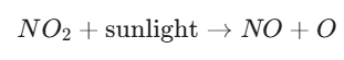
This leaves a highly reactive, single oxygen atom (O).

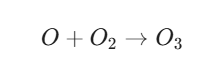
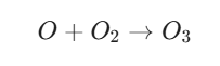
Step B: Ozone Formation

The free oxygen atom quickly binds with an oxygen molecule (O₂) already present in the atmosphere to form ozone:

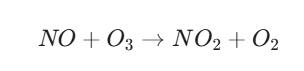
Step C: The “Scavenging” Reaction (The Balance)

In a clean environment, the leftover nitric oxide (NO) would react with the newly formed ozone to turn it back into NO₂ and O₂, keeping ozone levels low:

3. The Role of VOCs (The “Accelerator”)

If the cycle above were the only thing happening, ozone levels wouldn’t reach dangerous concentrations. VOCs disrupt the balance.

When VOCs are present, they react with other molecules to form peroxy radicals. These radicals “steal” the NO before it can react with the ozone.

Because the NO is “tied up” by the VOCs, it cannot “scavenge” or destroy the ozone formed in Step B.
As a result, ozone accumulates in the atmosphere rather than being converted back into O₂.

4. Environmental Factors

Because these reactions are driven by sunlight and heat, ozone concentrations are rarely constant:

Diurnal Patterns: Ozone levels typically peak in the mid-to-late afternoon when solar intensity is highest.
Seasonal Peaks: In the Northern Hemisphere, “Ozone Season” usually runs from May to September.
Stagnation: On hot, still days with little wind, these chemical “soups” sit over cities, allowing ozone concentrations to build up to hazardous levels, creating photochemical smog.

What is the story behind the smog in Southern Ontario and the British Columbia Lower Fraser Valley?

Wildfire smoke kills 1,500 Canadians per year –
CBC British Columbia and CBC News

The stories of Southern Ontario and the B.C. Lower Fraser Valley are two of the most significant case studies in Canadian atmospheric science. While both involve “smog,” the causes are vastly different: one is a story of continental transport, and the other is a story of geographic trapping.

1. Southern Ontario: The “Tail of the Tailpipe”

For decades, Southern Ontario (particularly the Windsor-Quebec City Corridor) was known as Canada’s smog capital.

The Transboundary Problem: Scientists discovered that much of Ontario’s air pollution wasn’t homegrown. It was being “imported” from the industrial heartland of the United States (the Ohio River Valley and the Midwest). Large coal-fired power plants and heavy industry released massive amounts of sulfur dioxide and nitrogen oxides.
The “Smog Summer” of 2005: This was a turning point. Ontario recorded a record 53 smog advisory days. The air was often a yellowish-brown haze, leading to increased hospital admissions for respiratory distress.
The Solution: The “story” here ended with a massive policy win. Ontario made the historic decision to phase out coal-fired power plants entirely (completed in 2014). This, combined with stricter vehicle emissions standards in both Canada and the U.S. (via the Canada-U.S. Air Quality Agreement), led to a dramatic decline in smog days. Today, most “smog” in Ontario is ground-level ozone on hot summer days, rather than the thick particulate smoke of the past.

2. Lower Fraser Valley, B.C.: The “Geographic Bowl”

The story in British Columbia is dominated by the unique topography of the Lower Fraser Valley (LFV).

The Trapping Effect: The LFV is shaped like a triangle, bounded by the Coast Mountains to the north and the Cascade Mountains to the southeast. When stable weather patterns occur, the mountains act like the walls of a bowl.
The Sea Breeze Cycle: During the day, the sun heats the land, drawing a sea breeze inland from the Strait of Georgia. This breeze pushes urban pollution from Vancouver and the surrounding cities eastward, deep into the valley toward Chilliwack and Hope.
Chemical Transformation: As the pollutants travel eastward, they have more time to react in the sunlight. This means that while the precursors are emitted in Vancouver, the highest concentrations of tropospheric ozone are often measured at the eastern end of the valley, far from the original source.
The Shift in Focus: In the 1990s, the concern was primarily vehicle exhaust. Today, the “new” smog story in the LFV is wildfire smoke. In recent summers, the “bowl” effect that used to trap car exhaust now traps thick woodsmoke, creating some of the worst temporary air quality readings in the world.

Comparison of the Two Regions

Feature	Southern Ontario	Lower Fraser Valley, B.C.
Primary Driver	Industrial & Transboundary (U.S.)	Topography & Local Transport
The “Wall”	None (open plains)	Coast and Cascade Mountains
Key Pollutant	SO₂ and O₃	O₃ and Fine Particulates (PM_2.5)
Typical Pattern	Long-range movement from SW	Diurnal “Sea-Breeze” cycle

What produces ozone in the stratosphere and how is air pollution affecting it and how will it affect life on Earth?

Climate 101: Ozone Depletion | National Geographic – National Geographic

While tropospheric ozone (smog) is a pollutant, stratospheric ozone is a vital “shield” that exists roughly 15 to 30 kilometers above the Earth. Its production and destruction are governed by a delicate chemical balance.

1. How Stratospheric Ozone is Produced

In the stratosphere, ozone is created naturally through the Chapman Cycle, a two-step process driven by high-energy ultraviolet (UV) radiation from the sun.

Step 1: Photolysis: High-energy UV-C light hits an oxygen molecule (O2), breaking the chemical bond and creating two free-roaming oxygen atoms

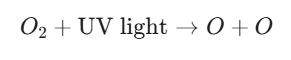
Step 2: Collision: These highly reactive oxygen atoms quickly collide and bind with other O2 molecules to form ozone (O3).

This process is most active over the tropics, where solar radiation is most intense, before atmospheric winds distribute the ozone globally.

2. How Air Pollution Affects the Ozone Layer

While natural processes also destroy ozone (keeping it in balance), certain human-made air pollutants act as catalysts that accelerate this destruction, leading to “thinning” or the famous “ozone hole.”

The Main Culprits (ODS): Chemicals known as Ozone-Depleting Substances (ODS)—specifically Chlorofluorocarbons (CFCs), Halons, and Hydrochlorofluorocarbons (HCFCs)—are the primary pollutants.
The Chain Reaction: When these stable chemicals reach the stratosphere, UV light breaks them down, releasing chlorine or bromine atoms. A single chlorine atom can destroy over 100,000 ozone molecules before it is eventually removed from the atmosphere.

(Notice the Cl is released at the end to start the cycle again.)

The 2026 Status: Thanks to the Montreal Protocol, the use of these chemicals has been phased out by nearly 99%. As of 2026, the ozone layer is officially in a state of healing. Scientists expect the “hole” over Antarctica to fully recover by roughly 2066, while the rest of the world may return to 1980 levels by 2040.

3. How Ozone Depletion Affects Life on Earth

The stratospheric ozone layer absorbs about 97% to 99% of the sun’s medium-frequency ultraviolet light (UV-B). Without this protection, life on Earth would face severe consequences:

Human Health: Increased UV-B radiation is directly linked to higher rates of skin cancer (melanoma and carcinomas) and cataracts. It can also suppress the human immune system, making us more vulnerable to infectious diseases.
Marine Ecosystems: UV-B penetrates several meters into the ocean, damaging phytoplankton, which form the base of the marine food web. It also harms the early developmental stages of fish, shrimp, and crabs.
Plant Life & Agriculture: High UV levels can alter plant physiological processes, reducing growth and total biomass. Studies suggest a 10% reduction in ozone could lead to a 6% decrease in global crop yields, threatening food security.+1
Material Degradation: UV radiation accelerates the breakdown of natural and synthetic polymers (like plastics and wood), leading to shorter lifespans for outdoor infrastructure and the increased creation of microplastics.

While the recovery of the ozone layer is a major environmental success story, the ongoing monitoring of “new” pollutants—such as emissions from increased rocket launches or certain unregulated industrial solvents—remains a priority for atmospheric scientists today.

What is the current air pollution levels and what are their trends?

What Is The Air Quality Index (AQI)? – Ecosystem Essentials –
Ecosystem Essentials

Current air pollution data from early 2026 shows a persistent gap between highly industrialized or rapidly developing regions and those with aggressive renewable energy policies. While some specific pollutants like nitrogen dioxide (NO₂) saw a temporary decline during the early 2020s, the global trend has largely rebounded, with nearly 99% of the world’s population breathing air that exceeds WHO guideline limits.

Current Global Air Quality Status (2026)

The primary metric used for global health assessments is PM_2.5 (particulate matter less than 2.5 micrometers in diameter).

Region/Rank	Most Polluted Countries (PM_2.5 avg)	Cleanest Countries (PM_2.5 avg)
1	Pakistan (67.3 μg/m³)	French Polynesia (1.8 μg/m³)
2	Bangladesh (66.1 μg/m³)	Puerto Rico (2.4 μg/m³)
3	Tajikistan (57.3 μg/m³)	Iceland (3.7 μg/m³)
4	Chad (53.6 μg/m³)	Australia (4.4 μg/m³)
5	India (48.9 μg/m³)	Estonia (4.7 μg/m³)

Hotspots: Central and South Asia remain the most affected regions due to a combination of vehicular emissions, seasonal agricultural burning, and industrial output.
WHO Compliance: Only about 14% of cities worldwide currently meet the WHO’s stringent annual average guideline for PM_2.5 (which is 5 μg/m³).

Key Global Trends

1. The Post-Pandemic Rebound

Global NO₂ levels—largely tied to traffic and fossil fuel combustion—showed a moderate decline between 2016 and 2019, followed by a sharp drop in 2020. However, data from 2023 through 2026 indicates a partial to full rebound in most urban centers as economic activity and transportation returned to pre-2020 levels.

2. Regional Divergence

Declining Trends: Major progress is being seen in regions like the Yangtze River Delta and Beijing-Tianjin-Hebei. Due to aggressive emission reduction policies, PM_2.5 levels in these areas have decreased by over 30 μg/m³ since 2016.
Rising Trends: Conversely, many low- and middle-income countries are seeing rising pollution levels. Rapid urbanization in Africa and parts of Southeast Asia, often coupled with older vehicle fleets and biomass fuel use, continues to drive up concentrations.

3. The Climate-Pollution Feedback Loop

Meteorology is playing an increasingly volatile role. Even in areas where emissions are being cut, “positive net anomalies” (increased pollution) are occurring due to stagnant weather patterns, reduced wind speeds, and temperature inversions—all of which are exacerbated by climate change. This means that to achieve the same air quality as ten years ago, cities must now cut emissions even more aggressively to counter these meteorological shifts.

4. Increased Focus on “Ultra-Fine” Particles

Global monitoring is shifting from PM₁₀ toward PM_2.5 and even PM_0.1 (ultrafine particles). These smaller particles are the leading environmental health risk globally, contributing significantly to non-communicable diseases and reduced life expectancy.

1. Where and Why Does it Happen?

While ozone depletion occurs globally, the most dramatic thinning happens over Antarctica during the Southern Hemisphere’s spring (September through November). This is due to a unique combination of extreme cold and atmospheric dynamics:

The Polar Vortex: During the dark winter months, a “whirlpool” of extremely cold air circles Antarctica, isolating the atmosphere there from the rest of the world.
Polar Stratospheric Clouds (PSCs): When temperatures drop below $-78\text{°C}$, rare clouds of ice and nitric acid form. These clouds provide a solid surface for inactive chlorine (from human-made CFCs) to turn into highly reactive chlorine gas.
The Sun’s Return: When the sun rises in the spring, the UV light hits that reactive chlorine, triggering a massive chain reaction that destroys ozone molecules at a rate of up to 1% per day.

2. The Role of Air Pollution

The primary cause of the ozone hole was the historical release of Chlorofluorocarbons (CFCs) and Halons. These were used in:

Refrigeration and air conditioning (Freon).
Aerosol spray cans.
Fire extinguishing systems.

Because CFCs are extremely stable, they do not wash out with rain or react in the lower atmosphere. Instead, they drift into the stratosphere over several years. Once there, they are broken apart by intense UV radiation, releasing the chlorine atoms that “eat” the ozone.

3. The Montreal Protocol and Recovery

The discovery of the ozone hole in the mid-1980s led to the Montreal Protocol (1987), which is widely considered the most successful environmental treaty in history.

Phase-Out: It mandated a global phase-out of ODS (Ozone Depleting Substances).
Current Status: As of April 2026, the ozone layer is in a steady state of healing. The “hole” still forms every year because the CFCs already in the atmosphere have very long lifetimes (50 to 100 years), but its average size and depth are gradually decreasing.

4. Why Should We Care?

The ozone layer is Earth’s “sunscreen.” Without it, the planet is exposed to excessive UV-B radiation, which causes:

Increased rates of skin cancer and cataracts in humans.
Damage to terrestrial plants and agricultural crops.
The death of phytoplankton, the foundation of the ocean’s food chain.

The ozone hole served as the first global proof that human-made chemical air pollution could fundamentally alter the Earth’s life-support systems on a planetary scale.

What factors affect air pollution?

What are the causes (and effects) of air pollution? –
One Sustainable Choice

Air pollution levels are never static; they are the result of a dynamic tug-of-war between emission sources and environmental factors that either trap or disperse those emissions.

The factors affecting air quality can be broken down into three main categories:

1. Meteorological Factors (Weather)

The atmosphere is not a passive container; it actively determines the fate of pollutants.

Wind Speed and Direction: Wind is the primary horizontal mover. High wind speeds dilute pollutants by mixing them with cleaner air, while “calm” conditions allow them to accumulate. Direction determines which communities—often those “downwind”—bear the brunt of industrial or traffic emissions.
Temperature Inversions: Normally, air cools as it rises. In an inversion, a layer of warm air sits on top of cooler air near the ground. This “cap” prevents vertical mixing, trapping pollutants in a concentrated layer where we breathe.
Sunlight (UV Radiation): Sunlight is the engine for secondary pollutants. It triggers the photochemical reactions that turn NO_x and VOCs into ground-level ozone (O₃).
Humidity and Precipitation: Rain and snow act as “scrubbers” through a process called wet deposition, physically washing particles and soluble gases (like SO₂) out of the sky.

2. Physical Factors (Topography)

The “shape” of the land dictates how air flows.

Basins and Valleys: Cities located in valleys (like the Lower Fraser Valley or Los Angeles) are prone to “geographic trapping.” Mountains act as physical barriers that block wind, making these areas highly susceptible to long-lasting inversion events.
Urban Canyons: In dense cities, tall buildings create “canyons” that can trap vehicle exhaust at street level, preventing the natural dispersion that would happen in a more open landscape.
Coastal Breezes: Near oceans, the daily cycle of land and sea breezes can either clear the air or, in some cases, recirculate pollutants back and forth between the coast and inland areas.

3. Human and Economic Factors (Anthropogenic)

These are the “input” factors that we have the most direct control over.

Industrial Density: The concentration of power plants, refineries, and factories in a specific area sets the “baseline” for primary pollutants like sulfur dioxide.
Transportation Volume: The “vehicle miles traveled” in a city is a direct driver of nitrogen dioxide and particulate matter levels.
Technological Shifts: The transition from coal-fired power to renewables or from internal combustion to electric vehicles represents a structural factor that can lower pollution levels even if population grows.
Regulatory Policy: Standards like the Canadian Ambient Air Quality Standards (CAAQS) dictate how much a facility is allowed to emit, effectively acting as a “ceiling” for local pollution levels.

Summary Table: Factors of Influence

Factor	Effect on Pollution	Typical Result
High Wind Speed	High Dispersion	📉 Lower Concentration
Temperature Inversion	High Trapping	📈 Higher Concentration
Heavy Rainfall	Wet Deposition	📉 Lower Concentration
Valley Topography	Physical Containment	📈 Higher Concentration
High UV Index	Chemical Reaction	📈 Higher Ozone (O₃)

Understanding these factors is why air quality forecasting is so complex—it’s not just about how much we emit, but what the Earth does with those emissions once they leave the stack or tailpipe.

How does wind affect air pollution?

M2 L2 Importance of wind circulation in air pollution – Prof. Pratap Sonavane

Wind is the primary mechanism for the movement and dilution of air pollutants. Its influence is categorized by speed, direction, and the turbulence it creates.

1. Wind Speed: Dilution and Dispersion

Wind speed determines the volume of air available to “wash away” or dilute a pollutant at its source.

The High-Speed “Dilution” Effect: Faster winds stretch a plume of smoke or exhaust over a larger area, reducing the concentration of pollutants in any single spot. This is why windy days often have much lower AQHI (Air Quality Health Index) values.
The Low-Speed “Accumulation” Effect: When winds are stagnant (less than 5–10 km/h), pollutants linger near their source. This lack of “ventilation” leads to high-pollution episodes, particularly in urban areas during rush hour.

2. Wind Direction: The Path of Exposure

Wind direction dictates which communities are “downwind” of a source.

Source Tracking: Meteorologists use wind direction data to trace high pollution readings back to specific industrial zones or highways.
Transboundary Transport: Wind doesn’t respect borders. Prevailing winds can carry sulfur and nitrogen emissions hundreds of kilometers. For example, prevailing southwesterly winds can carry industrial pollutants from the U.S. Midwest into Southern Ontario and Quebec.+1

3. Turbulence: Mixing the “Chemical Soup”

Wind doesn’t just move air horizontally; it creates “eddies” and swirls that mix air vertically.

Mechanical Turbulence: Caused by wind moving over physical obstacles like buildings or mountains. These eddies help “scrub” the air by mixing surface-level pollution with cleaner air from higher up.
Thermal (Convective) Turbulence: On sunny days, the ground heats the air, causing it to rise. This creates vertical “conveyor belts” that pull pollutants away from the street level and lift them high into the troposphere.

4. Topography and Wind Interactions

In complex landscapes, wind behaves in ways that can either protect or endanger local air quality:

Valley Trapping: In regions like the Lower Fraser Valley, mountains act as barriers. If the wind isn’t strong enough to push air over the ridges, pollutants get trapped in the valley floor, circling in a stagnant “bowl.”
Urban Canyons: In downtown Calgary or other dense cities, tall buildings can channel wind at high speeds (the “Venturi effect”) or create stagnant pockets behind structures where vehicle exhaust can reach dangerous levels despite a windy day overall.

Summary of Wind’s Effect

Condition	Effect on Pollution	Typical Result
High Wind Speed	High Dilution	📉 Better Air Quality
Calm Winds	High Accumulation	📈 Poorer Air Quality
Stable Atmosphere	Limited Vertical Mixing	⚠️ Risk of Smog / Inversion
Rough Terrain	Increased Turbulence	🔄 Enhanced Mixing

Understanding wind patterns is essential for your work in meteorology and website forecasting tools, as it allows for the prediction of where a “plume” will move before it even reaches a monitoring station.

How does atmospheric stability and inversions affect air pollution?

How inversions affect pollution and air quality –
KTVB

Atmospheric stability and inversions are the “traffic controllers” of the sky. They determine whether the pollutants we emit will rise and vanish into the upper atmosphere or stay trapped at the surface where we breathe.

1. The Concept of Atmospheric Stability

Stability refers to the atmosphere’s resistance to vertical motion. It is measured by comparing the Environmental Lapse Rate (ELR)—the actual change in temperature with height—against the Dry Adiabatic Lapse Rate (DALR), which is the rate at which a dry air parcel cools as it rises (9.8°C per km).

Unstable Atmosphere (The “Elevator”)

Condition: The ground is warm, and air temperature drops rapidly with height (Super-adiabatic).
Effect: A parcel of air that starts rising stays warmer than the surrounding air, so it keeps moving upward like a hot air balloon.
Result for Pollution: Excellent dispersion. Pollutants are carried high into the sky and diluted quickly.

Stable Atmosphere (The “Resistance”)

Condition: Air temperature drops very slowly with height, or stays the same (Sub-adiabatic).
Effect: If a parcel of air tries to rise, it quickly becomes cooler and denser than its surroundings and sinks back down.
Result for Pollution: Poor dispersion. Pollutants “hang” in the air near their source, leading to hazy skies and rising AQHI levels.

2. Temperature Inversions: The “Atmospheric Lid”

A temperature inversion is the most extreme form of atmospheric stability. Instead of getting colder with height, the air actually gets warmer. This creates a layer of warm air that sits like a physical lid over cooler, denser air at the surface.

Types of Inversions

Radiation Inversion: Common on clear, calm nights when the ground loses heat rapidly. By morning, a shallow layer of cold air is trapped at the surface. These usually break up once the sun heats the ground.
Subsidence Inversion: Associated with high-pressure systems (anticyclones). Sinking air from above warms up as it is compressed, creating a massive warm layer aloft. These can last for days, leading to major “smog episodes.”

3. The Impact on Pollution Dispersion

Stability directly dictates the shape and behavior of smoke plumes from stacks:

Stability Class	Plume Type	Behavior
Highly Unstable	Looping	Plume moves up and down in large “loops.” Good for long-distance dilution but can cause high concentrations if a loop hits the ground.
Neutral	Coning	Plume spreads out in a cone shape. Moderate dispersion.
Stable	Fanning	Plume stays in a thin, flat layer and travels long distances horizontally without mixing vertically.
Inversion	Fumigation	A dangerous scenario where a plume is released below an inversion; it cannot go up, so it is forced downward toward the ground.

Why it Matters in Western Canada

The science behind temperature inversions – Washington Department of Ecology

In regions like the Lower Fraser Valley or deep in the Alberta Prairies during winter, cold air often pools in low-lying areas while warm air passes overhead. This creates a “perfect trap” for vehicle exhaust and woodsmoke. During these inversions, even small amounts of pollution can build up to unhealthy levels in just a few hours because the “room” (the volume of air available for mixing) has been made much smaller by the inversion lid.

What is a temperature inversion?

This video explains the mechanics of how a layer of warm air acts as a lid to trap wood smoke and car exhaust at ground level during the winter.

What is indoor air pollution?

What is Indoor Air Quality? –
Paul Cochrane

Indoor air pollution refers to the chemical, physical, or biological contamination of air within a building or enclosed space. It is a critical health concern because the concentration of pollutants indoors can be 2 to 5 times higher than outdoor levels, and most people spend approximately 90% of their time inside.

1. Common Indoor Pollutants and Sources

Indoor air quality (IAQ) is affected by a mix of “homegrown” contaminants and outdoor pollutants that have migrated inside.

Combustion Byproducts: Sources like gas stoves, wood-burning fireplaces, and tobacco smoke release carbon monoxide (CO), nitrogen dioxide (NO₂), and fine particulate matter (PM_2.5).
Volatile Organic Compounds (VOCs): These are gases emitted from common household products like paints, cleaning supplies, new furniture, and carpets. They evaporate at room temperature and can cause headaches or long-term organ damage.
Biological Contaminants: This category includes mold, pet dander, dust mites, and pollen. Moisture control is the primary factor in preventing mold growth, which is a significant respiratory irritant.
Radon Gas: A naturally occurring radioactive gas that seeps into buildings through foundation cracks. It is the second leading cause of lung cancer after smoking.
Building Materials: Older structures may still contain asbestos or lead dust, which become hazardous when disturbed during renovations.

2. Why Does It Accumulate?

The severity of indoor pollution is often tied to a building’s Air Exchange Rate.

Tight Seals: Modern energy-efficient homes are often “sealed” to prevent heat loss. Without mechanical ventilation, pollutants have no way to escape and build up over time.
HVAC Performance: If an HVAC system is poorly maintained or has clogged filters, it can circulate dust and mold rather than cleaning the air.
Infiltration: During high-pollution events outside (like the 2025 wildfire season), outdoor smoke can penetrate indoor spaces through gaps in windows and doors.

3. Health Impacts

Because we spend so much time indoors, chronic exposure to low levels of these pollutants can be more damaging than short-term outdoor spikes.

Immediate Effects: Irritated eyes, nose, and throat; headaches; dizziness; and fatigue. These are often categorized as Sick Building Syndrome.
Long-Term Risks: Respiratory diseases (like asthma), heart disease, and impaired cognitive function.
Vulnerable Groups: Children, the elderly, and those with pre-existing conditions are at the highest risk, especially since they typically spend the most time at home.

4. 2026 Trends in Indoor Air Quality

As of 2026, the focus on IAQ has shifted toward smarter, data-driven solutions:

Smart HVAC Systems: New systems now use real-time sensors to detect $CO_2$ and VOC levels, automatically increasing ventilation when air quality dips.
Electrification: There is a growing trend of replacing gas-fired appliances with electric induction stoves and heat pumps to eliminate indoor combustion sources.
Portable HEPA Filtration: High-Efficiency Particulate Air (HEPA) filters have become a household staple, capable of removing 99.97% of particles as small as 0.3 microns.

Strategy	Action	Benefit
Source Control	Switch to low-VOC paints; stop smoking indoors.	Most effective way to reduce pollution.
Ventilation	Open windows; use kitchen exhaust fans.	Dilutes and removes stale air.
Air Cleaning	Use HEPA purifiers or high-MERV HVAC filters.	Removes particulates like dust and smoke.

What are smokestack plumes?

Air Pollution Lesson 08E: Steam vs. Particle Plumes –
John Cimbala

Smokestack plumes are the visible (or sometimes invisible) streams of gases, particulate matter, and heat released from an industrial chimney into the atmosphere. The shape and behavior of these plumes are a primary focus of atmospheric science, as they reveal exactly how the atmosphere is moving at that specific location.

The way a plume behaves—whether it rises, sinks, or spreads—is determined by the interaction between the buoyancy of the gases and the stability of the surrounding air.

1. The Physics of the Plume

A plume goes through three distinct stages after it leaves the stack:

The Rise Stage: Because the gases are usually much hotter than the surrounding air, they are less dense and rise quickly due to buoyancy.
The Interaction Stage: As the plume rises, it begins to mix with the ambient air (entrainment). Its momentum and heat are shared with the atmosphere.
The Dispersion Stage: Once the plume’s temperature matches the surrounding air, its upward motion stops, and it begins to move horizontally with the prevailing wind.

2. Plume Shapes and Atmospheric Stability

Meteorologists categorize plumes by their shape, as these shapes act as a visual “signature” of the vertical temperature profile of the atmosphere.

Looping Plume

Occurs in highly unstable conditions (usually hot, sunny days). Large thermal eddies in the air push the plume up and down in a wavy, looping pattern.

Impact: While it dilutes quickly, it can occasionally “loop” down to the ground, causing high localized concentrations of pollutants.

Coning Plume

Occurs in neutral stability conditions (often cloudy days or high winds). The plume spreads out in a steady, symmetric cone shape.

Impact: This is the “ideal” behavior for standard dispersion models.

Fanning Plume

Occurs during an inversion or very stable conditions. Because the air cannot move vertically, the plume stays in a thin, flat layer that can travel for many kilometers without spreading out.

Impact: Little pollution reaches the ground near the stack, but the plume can stay concentrated for long distances.

Fumigation

This is the most hazardous scenario. It occurs when a plume is released into a stable layer, but a turbulent, unstable layer exists just below it (often during the morning as the sun begins to heat the ground).

Impact: The “lid” above prevents the plume from rising, while the turbulence below “pulls” the entire concentrated plume down to the surface at once.

3. Factors Affecting Plume Height

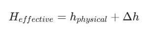
To minimize the health impact on nearby communities, engineers aim for the highest “effective stack height.” This is calculated using two variables:

Physical Stack Height: The actual height of the chimney.
Plume Rise (Δh): The extra height the gases gain due to their exit velocity and temperature.

In the context of meteorological data and website tools, understanding these behaviors is essential for Dispersion Modeling, which predicts how an industrial event in one area might affect the air quality in another.

How does topography affect air pollution?

Topography—the physical shape and features of the land—acts as a secondary “container” for the atmosphere. It can either facilitate the rapid cleaning of the air or create physical traps that allow pollutants to reach dangerous concentrations.

For a professional in Geomatics and Meteorology, topography is often the most critical variable in determining why two cities with identical emissions can have vastly different air quality profiles.

1. The “Bowl” Effect (Basins and Valleys)

In flat terrain, wind can move freely to disperse pollutants. In mountainous or hilly terrain, the land acts as a physical barrier.

Physical Blockage: Mountains block the horizontal flow of air. If a city is located in a valley, pollutants from cars and industry can’t be “blown away” easily.
Cold Air Pooling: At night, cold air (which is denser) flows down mountain slopes and settles on the valley floor. This creates a highly stable environment where pollutants are pinned to the ground.
The Case of the Lower Fraser Valley: As we discussed, the “triangle” of mountains surrounding this region creates a classic topographic trap that funnels and holds ozone and particulates.

2. Thermally Driven Slope Winds

Topography creates its own local wind systems that can move pollution in predictable daily cycles.

Anabatic Winds (Daytime): As mountain slopes are heated by the sun, air rises up the slopes. This can pull pollution out of a valley floor and transport it to higher elevations, affecting alpine ecosystems.
Katabatic Winds (Nighttime): As slopes cool, the air becomes dense and “falls” back into the valley. This can concentrate pollutants from higher-elevation sources (like mountain-side homes with wood stoves) back down into populated valley centers.

3. Urban Topography (The “Urban Canyon”)

On a smaller scale, the “topography” of a city—its buildings—creates a microclimate.

The Venturi Effect: Tall buildings can funnel wind into narrow streets, increasing speed but also creating “dead zones” behind structures where air remains stagnant.
Street Canyons: In deep urban canyons, vehicle exhaust is often trapped at the sidewalk level. The buildings prevent the wind from reaching the street to “flush” the air, leading to much higher NO₂ levels at the ground than what a rooftop monitor might suggest.

4. Coastal Topography and Sea Breezes

When mountains are located near a coastline, they interact with the sea breeze to create a “recirculation” effect.

Recirculation: During the day, the sea breeze pushes urban pollution toward the mountains. At night, the land breeze pushes it back out toward the water. However, if the mountains are high enough, the pollution can get caught in a loop, moving back and forth over the city for several days without ever being fully dispersed into the open atmosphere.

Summary of Topographic Influence

Feature	Primary Mechanism	Air Quality Result
Deep Valley	Cold air pooling & Physical barriers	📈 High risk of prolonged smog episodes.
Steep Slopes	Katabatic/Anabatic wind cycles	🔄 Daily “sloshing” of pollutants.
Urban Canyons	Mechanical turbulence & Shielding	⚠️ High localized exposure at street level.
Coastal Ridges	Sea-breeze interaction	🔄 Risk of pollutant recirculation.

Is there a way to measure the potential for severe air pollution events?

Explaining air quality measurements and how agencies report numbers – KREM 2 News

Measuring the potential for a severe air pollution event involves looking at the atmospheric capacity—essentially determining how much “room” the atmosphere has to dilute emissions before they reach dangerous concentrations.

Meteorologists and environmental scientists use several quantitative indices and physical models to predict these events.

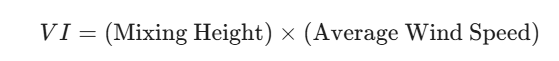
1. Ventilation Index (VI)

In Canada, this is the most common tool used to determine if the atmosphere can disperse smoke and pollutants. It is a calculated value based on two primary variables:

Mixing Height: The height above the surface where vigorous vertical mixing occurs. If the mixing height is low (e.g., under 500 meters), pollutants are trapped near the ground.
Average Wind Speed: The average speed within that mixing layer.

The formula for the Ventilation Index is generally expressed as:

Interpretation of VI:

Poor (0–33): Very little movement; pollutants will accumulate rapidly.
Fair (34–54): Moderate dispersion; limited burning or industrial activity may be allowed.
Good (55–100): High capacity for dispersion; the atmosphere can easily “flush” emissions.

2. Dispersion Modeling (AERMOD and CALPUFF)

Rather than just looking at the general state of the air, dispersion models predict the specific path and concentration of a pollutant plume.

AERMOD: The standard regulatory model used for short-range dispersion (within 50 km). It uses boundary layer turbulence and terrain data to predict ground-level concentrations.
CALPUFF: Used for long-range transport (over 50 km). It is particularly effective in regions with complex topography, like the BC mountains or the Alberta foothills, because it can model how a “puff” of pollution bends and flows around physical obstacles.

3. The Pasquil Stability Classes

Scientists categorize the “potential” for pollution using the Pasquill-Gifford stability classes, labeled A through F.

Class A (Highly Unstable): High potential for dispersion (low pollution risk).
Class F (Highly Stable): High potential for a severe pollution event (high risk).

During a Class F event, usually occurring on a calm, clear night with a temperature inversion, the atmosphere is “closed,” and even a small amount of wood smoke or vehicle exhaust can lead to a rapid spike in the AQHI (Air Quality Health Index).

4. Synoptic Weather Patterns

On a larger scale, meteorologists look for specific “setups” on weather maps:

Stagnant High-Pressure Systems: Large “H” cells on a map often mean sinking air (subsidence) and light winds. If a high-pressure system parks over a region for several days, it creates a “pollution clock” that ticks toward a severe event.
Upper-Level Ridges: These often lead to the formation of subsidence inversions, which act as a heavy lid over entire provinces.

5. Automated Monitoring Networks

Finally, we measure potential by looking at real-time trends from ground stations. In the Calgary area, organizations like the Calgary Region Airshed Zone (CRAZ) monitor:

Concentration Trends: If NO₂ or PM_2.5 levels are climbing steadily while wind speeds are dropping, it serves as an early warning of a coming event.
Lidar Vertical Profiling: Using laser light to detect the exact height of the inversion layer in real-time.

What factors affect urban air pollution?

How Winter Conditions Can Contribute to Poor Urban Air Quality – The Weather Network

Urban air pollution is a unique “cocktail” of chemicals and particles that is far more concentrated than in rural areas. While the sources (cars and industry) are obvious, several structural and meteorological factors determine whether a city’s air remains breathable or becomes a health hazard.

1. Urban Morphology (The “Urban Canyon”)

The physical layout of a city—its “geometry”—is one of the most significant factors.

Building Density: When tall buildings line both sides of a narrow street, they create an urban canyon. This prevents crosswinds from reaching the street level, trapping vehicle exhaust exactly where pedestrians are walking.
Aspect Ratio: The ratio of building height to street width determines how much air can circulate. In deep canyons, the air can become stagnant for hours.
Surface Roughness: On a broader scale, a city of varying building heights creates “drag” on the wind, slowing down the overall ventilation of the metropolitan area.

2. The Urban Heat Island (UHI) Effect

Cities are significantly warmer than their rural surroundings because concrete and asphalt absorb solar radiation.

Thermal Circulations: The extra heat creates a “heat dome.” Warm air rises over the city center, which can actually pull in pollutants from surrounding industrial suburbs in a localized “country-to-city” breeze.
Chemical Acceleration: Higher temperatures speed up the photochemical reactions that produce ground-level ozone (O₃). This is why smog is often worst during urban heatwaves.

3. Transportation and Traffic Patterns

In most modern cities, mobile sources are the primary contributors to poor air quality.

Cold Starts: Engines are least efficient when they first start. In dense residential areas, “cold start” emissions in the morning can lead to localized spikes in CO and NO₂.
Idling and Congestion: Stop-and-go traffic increases the volume of pollutants per kilometer traveled.
Non-Exhaust Emissions: As we move toward electric vehicles, tailpipe emissions are dropping, but brake wear, tire wear, and road dust remain significant sources of particulate matter (PM₁₀).

4. Local Topography and Wind

A city’s geographic “bed” plays a massive role in its pollution potential.

Basin Effects: Cities like Los Angeles or Mexico City are in geographic basins that act as natural bowls, making it nearly impossible for pollutants to escape when winds are light.
Sea and Lake Breezes: For coastal cities, the daily shift in wind direction can recirculate pollution. During the day, the sea breeze pushes smog inland; at night, the land breeze pushes it back out, often trapping the same air mass over the city for days.

5. Summary of Urban Factors

Factor	Mechanism	Result
Urban Canyons	Limits horizontal ventilation	📈 High street-level NO₂ and CO.
Heat Island	Increases reaction speed	📈 Higher summer ozone (O₃) levels.
Congestion	Increases emission duration	📈 Higher particulate matter (PM_2.5).
Topography	Physical containment	⚠️ Risk of “multi-day” smog events.

Is there a relationship between heat domes and air pollution and can heat waves make air pollution better or worse?

Extreme Heat & Air Pollution Connection Explained | Climate Change Impact on Health & Cities –
Clean Copper Talks

There is a direct and dangerous relationship between heat domes and air pollution. In atmospheric science, a heat dome acts as a “pressure cooker” for pollutants, and while heat waves can technically “clear” the air in very specific circumstances, they almost universally make air quality significantly worse.

1. The Heat Dome as an Atmospheric Trap

A heat dome occurs when a high-pressure system stalls over a large area, trapping hot air underneath it. This affects pollution in three specific ways:

Subsidence (The Lid): In a high-pressure system, air sinks. This sinking air (subsidence) acts like a heavy, invisible lid that prevents pollutants from rising and dispersing. This is often accompanied by a subsidence inversion, where a layer of warm air sits on top of cooler air near the ground, pinning exhaust and smoke at breathing level.
Stagnation: Heat domes are characterized by very light winds. Without wind to “flush” the city, the pollutants emitted by cars and industry simply pool and concentrate in the same location day after day.
The “Chemical Kitchen”: High temperatures and intense sunlight within a heat dome act as a catalyst. This speeds up the photochemical reactions between nitrogen oxides (NO_x) and volatile organic compounds (VOCs), leading to a rapid spike in ground-level ozone (O₃).

2. Can Heat Waves Ever Make Air Pollution Better?

While it seems counterintuitive, there is one specific scenario where extreme heat can temporarily improve surface air quality: Deep Vertical Mixing.

If a heat wave is “dry” and the ground becomes exceptionally hot, it can create intense thermal turbulence. This can break through a shallow inversion layer, essentially “punching a hole” in the lid and allowing surface pollutants to be carried high into the troposphere. In this case, while the air might be dangerously hot, the concentration of particulates at the street level might actually drop as they are sucked upward.

3. Why Heat Waves Usually Make Air Pollution Worse

In the vast majority of cases, the “clearing” effect mentioned above is overwhelmed by these negative factors:

Natural Emissions: As temperatures rise, trees and plants actually release more biogenic VOCs (like isoprene and terpenes) as a stress response. These natural chemicals react with man-made pollution to create even more ozone.
Wildfire Feedback: Extreme heat waves dry out vegetation (fuel), making wildfires more likely. The resulting wood smoke introduces massive amounts of fine particulate matter (PM_2.5) that can travel thousands of kilometers.
Increased Energy Demand: During a heat wave, the demand for air conditioning skyrockets. This forces power plants to run at maximum capacity, often increasing the emissions of sulfur dioxide (SO₂) and nitrogen oxides (NO_x) at the very time the atmosphere is least able to disperse them.
Evaporative Emissions: Higher temperatures increase the rate at which gasoline and industrial solvents evaporate, adding more raw material to the smog-building process.

Summary: The Heat-Pollution Penalty

Factor	Effect of Heat Wave	Impact on Air Quality
Wind Speed	Often decreases (stagnation)	📈 Worse (accumulation)
Atmospheric Lid	Subsidence inversion forms	📈 Worse (trapping)
Chemical Reactions	Reaction rates double/triple	📈 Worse (high ozone)
Biogenic VOCs	Plants release more gas	📈 Worse (more smog precursors)
Thermal Mixing	Can break shallow inversions	📉 Better (rare/temporary)

What is acid deposition?

What is Acid Rain? | National Geographic –
National Geographic

Acid deposition, commonly known as “acid rain,” refers to any form of precipitation—including rain, snow, fog, hail, or even dry dust—that has an unusually low pH (is more acidic than normal).

While natural rainwater is slightly acidic (with a pH of about 5.6) due to dissolved carbon dioxide, acid deposition typically has a pH between 4.2 and 4.4.

1. The Chemical Process

Acid deposition is a secondary pollution process. It begins when two primary pollutants are released into the atmosphere:

Sulfur Dioxide (SO₂): Primarily from coal-fired power plants and metal smelters.
Nitrogen Oxides (NO_x): Primarily from vehicle exhaust and industrial boilers.

When these gases are lofted into the atmosphere, they react with water, oxygen, and other chemicals to form sulfuric acid (H₂SO₄) and nitric acid (HNO₃). These acids then fall to the ground in two ways:

Wet Deposition: The acids mix with rain, snow, or fog and fall to the surface.
Dry Deposition: In dry areas, the acidic pollutants stick to dust or smoke and settle on the ground, buildings, or vegetation. When the next rain occurs, these dry particles mix with water to form a highly acidic runoff.

2. Environmental Impacts

Acid deposition doesn’t just “burn” things on contact; it changes the fundamental chemistry of ecosystems:

Aquatic Life: Most fish eggs cannot hatch at a pH below 5. As lakes become more acidic, “aluminum leaching” occurs—acid rain pulls aluminum from the soil into the water, which is toxic to fish and clogs their gills.
Forests: Acid rain dissolves vital nutrients (like calcium and magnesium) from the soil before trees can use them. It also damages the protective waxy coating on leaves, making trees more susceptible to disease and extreme cold.
Soil Chemistry: In areas like the Canadian Shield, where the bedrock is granite and has low “buffering capacity,” the soil cannot neutralize the acid, leading to rapid ecosystem decline.
Architecture: Acid rain reacts with minerals in limestone, marble, and sandstone. This causes statues, historic buildings, and gravestones to dissolve and “crumble” over time.

3. The “Success Story” of the 1990s

Acid rain was the primary environmental crisis of the 1970s and 80s, especially in Eastern Canada.

The Problem: High-altitude winds carried SO₂ from the U.S. Ohio River Valley into Ontario and Quebec, “killing” thousands of lakes.
The Policy: This led to the Canada-U.S. Air Quality Agreement (1991). By mandating “scrubbers” on smokestacks and switching to low-sulfur fuels, SO₂ emissions in North America have dropped by over 90% since 1990.

4. Current Status in 2026

While SO₂ levels are significantly lower, scientists are now focused on Nitrogen Deposition. Nitrogen oxides from transportation are still a major factor, and while they are less “acidic” than sulfur, they act as an unwanted fertilizer in lakes, leading to algae blooms and decreased oxygen levels.

Cavanu Starline Air Pollution Calculator

Solved Problems

Here are 20 high-level application problems centered on air pollution meteorology and atmospheric chemistry, designed to test reasoning and reasoning-based problem-solving skills.

Atmospheric Dispersion and Stability Problems

1. Problem: A power plant with a 100m stack is located in a valley. During the night, the ground cools rapidly. Will the dispersion of pollutants likely be better or worse than during the day?

Reasoning: Nighttime cooling leads to a temperature inversion (stable air). Inversions suppress vertical mixing, trapping pollutants near the surface.
Solution: Dispersion will be worse due to suppressed vertical mixing and lack of thermal turbulence.

2. Problem: A chemical spill occurs during a sunny afternoon (Class B stability) versus a cloudy, windy night (Class D stability). Where will the plume reach the ground first?

Reasoning: Class B (unstable) is characterized by convective updrafts and downdrafts. Class D (neutral) relies on mechanical turbulence. Unstable air forces the plume to the ground more rapidly via turbulent eddies.
Solution: Class B. The instability forces the plume down quickly.

3. Problem: You are modeling a plume using the Gaussian model. If wind speed (u) doubles while emissions (Q) remain constant, what happens to the ground-level concentration (C)?

Reasoning: The Gaussian plume equation shows concentration is inversely proportional to wind speed.
Solution: Concentration will be reduced by half.

4. Problem: Why does a “looping” plume occur primarily on sunny days with light winds?

Reasoning: Large convective cells (thermal eddies) break up the plume into discrete “loops” as it moves downwind.
Solution: Strong solar heating creates thermal instability, forcing the plume to move with large convective eddies.

5. Problem: Compare a “fanning” plume to a “lofting” plume in terms of environmental impact.

Reasoning: Fanning happens in stable air; lofting happens when the atmosphere is unstable above the stack but stable below.
Solution: Fanning keeps the plume aloft (minimal ground impact); lofting keeps the plume aloft due to a stable surface layer, making both relatively safe for ground-level receptors.

Pollutant Concentration and Chemistry

6. Problem: Calculate the ppm concentration of SO₂ if the measured concentration is 50 mg/m³ at 25°C and 1 atm. (Molar mass of SO₂ = 64.06 g/mol).

Reasoning: Use the conversion formula: ppm = (mg/m³ * 24.45) / (Molar Mass).
Solution: (50 * 24.45) / 64.06 ≈ 19.09 ppm.

7. Problem: A city switches from coal to natural gas. Which primary air pollutant will likely see the largest reduction?

Reasoning: Coal contains significant sulfur and particulate matter. Natural gas is cleaner but still produces NO_x.
Solution: Sulfur Dioxide (SO₂) and Particulate Matter (PM_2.5).

8. Problem: What is the limiting reagent in the production of photochemical smog in an urban environment?

Reasoning: Smog requires NO_x, VOCs, and sunlight. Usually, VOCs are the limiting reagent in urban centers.
Solution: Volatile Organic Compounds (VOCs).

9. Problem: If relative humidity is very high, how does this affect the conversion of SO₂ to sulfuric acid (H₂SO₄)?

Reasoning: High humidity provides liquid water on aerosol surfaces, facilitating aqueous-phase oxidation.
Solution: It accelerates the conversion rate significantly through aqueous chemistry.

10. Problem: Why does the ozone (O₃) concentration in a city center often drop during the morning rush hour?

Reasoning: Freshly emitted NO from vehicles reacts with existing O₃ to form NO₂ (titration effect).
Solution: NO titration consumes O₃ near high-traffic areas.

Meteorological and Boundary Layer Dynamics

11. Problem: An air parcel is lifted from the surface. If the Environmental Lapse Rate (ELR) is 12°C/km and the Dry Adiabatic Lapse Rate (DALR) is 9.8°C/km, is the atmosphere stable or unstable?

Reasoning: If ELR > DALR, the parcel remains warmer than the surroundings and keeps rising.
Solution: Unstable.

12. Problem: Define the “mixing height” and its importance to pollution.

Reasoning: It is the height to which surface emissions are vertically mixed.
Solution: It defines the volume of air available to dilute pollutants; a lower height equals higher concentrations.

13. Problem: How does a “heat island” effect influence air quality?

Reasoning: Cities are warmer than rural areas, creating localized convection.
Solution: It can induce a local circulation that traps pollutants or promotes vertical dispersion depending on the synoptic flow.

14. Problem: Why is NO₂ typically higher in the winter than in the summer in mid-latitude cities?

Reasoning: Lower solar intensity leads to slower photochemical destruction of NO_x.
Solution: Reduced photolysis rates in winter increase the atmospheric lifetime of NO_x.

15. Problem: Describe the effect of a sea breeze on the concentration of pollutants in a coastal city.

Reasoning: Daytime sea breezes push air from the water to the land.
Solution: It can recirculate pollutants, trapping them in a “loop” between land and sea, increasing ground levels.

Advanced Reasoning

16. Problem: If you double the stack height (H), the ground-level concentration (C) decreases significantly. Why is this not a “magic bullet” for all pollutants?

Reasoning: While it reduces local ground impact, it increases long-range transport and contributes to acid rain or transboundary pollution.
Solution: It disperses pollutants over a larger geographical area, potentially causing regional rather than local issues.

17. Problem: How do “secondary aerosols” form in the atmosphere?

Reasoning: Gaseous precursors (SO₂, NO_x, VOCs) undergo chemical reactions to form particles.
Solution: Chemical reaction and subsequent condensation/nucleation of gases into solid or liquid particles.

18. Problem: Why is the PM_2.5/PM₁₀ ratio higher in urban areas compared to rural areas?

Reasoning: Urban sources (combustion) produce finer particles; rural sources (dust) produce coarser particles.
Solution: Combustion emissions are inherently finer (sub-micron) than mechanical dust.

19. Problem: What meteorological condition is required for the formation of “London Smog” (sulfurous smog)?

Reasoning: High humidity + stagnation + sulfur emissions.
Solution: A surface-based radiation inversion combined with light winds and high relative humidity.

20. Problem: If we successfully eliminate all NO_x emissions, what happens to the ozone concentration?

Reasoning: Ozone chemistry is non-linear; in very high NO_x environments, NO_x can actually suppress ozone.
Solution: In extreme NO_x saturation zones, ozone levels might actually rise briefly before falling as the system shifts toward a VOC-limited regime.

Air Pollution Quiz | Local Scope Edition

Air Pollution Quiz

Test your knowledge on atmospheric stability, inversions, and global trends.

Results

What is weather in the context of climate and the environment?

Earth and Atmospheric Sciences

What is air pollution?