Why is the earth’s climate changing?

Earth’s climate is currently changing primarily due to an enhanced greenhouse effect caused by human activities. While the Earth has gone through natural cycles of warming and cooling over millions of years, the current rate of change is unprecedented in the last several thousand years.

The Greenhouse Effect

Under natural conditions, certain gases in our atmosphere act like the glass of a greenhouse. They allow sunlight to enter but trap some of the heat radiating back from the Earth’s surface, keeping our planet warm enough to support life.

Greenhouse effect – Wikipedia

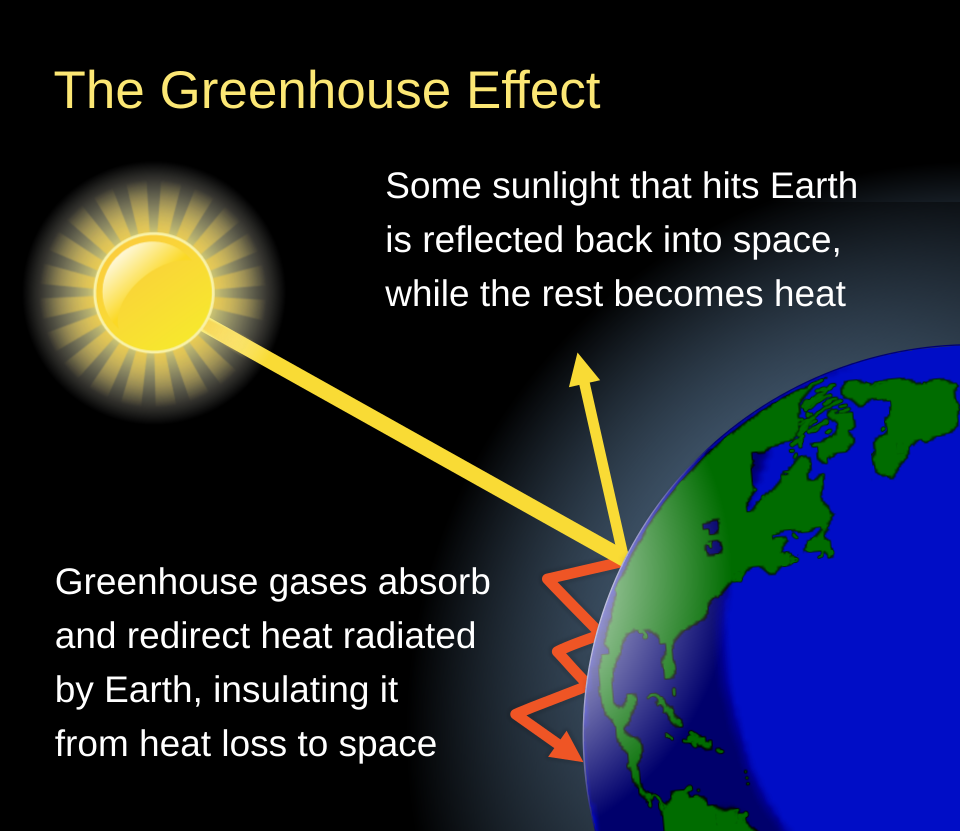
However, human activity has significantly increased the concentration of these gases, effectively “thickening the blanket” around the planet and trapping excess heat. The primary gases responsible include:

Carbon Dioxide (CO₂): Released through the burning of fossil fuels (coal, oil, and natural gas) for electricity, manufacturing, and transportation.
Methane (CH₄): Emitted during the production and transport of coal, gas, and oil, as well as from livestock and agricultural practices.
Nitrous Oxide (N₂O): Primarily a result of agricultural activities and industrial processes.

Primary Drivers of Rising Emissions

AeroStat Prime – Canavu Starline

The increase in these gases is tied to several core sectors of modern society:

Generating Power: Most electricity is still produced by burning fossil fuels, which releases massive amounts of CO₂ and N₂O.
Manufacturing & Industry: The production of cement, iron, steel, and electronics requires intense energy, often derived from carbon-heavy sources.
Deforestation: Trees absorb CO₂. When they are cut down or burned, they not only stop absorbing carbon but also release the carbon they have stored back into the atmosphere.
Transportation: Most cars, ships, and planes rely on petroleum-based fuels like gasoline and diesel.
Food Production: Large-scale agriculture involves clearing land, using synthetic fertilizers, and raising livestock—all of which contribute to greenhouse gas output.

Scientific Evidence and Feedback Loops

As the planet warms, “feedback loops” can accelerate the process. For example, as Arctic sea ice melts, the darker ocean water absorbs more sunlight than the reflective white ice did, leading to even further warming.

Data from 2026 shows that atmospheric CO₂ levels are higher than they have been in over 2 million years. This shift is disrupting weather patterns, causing more frequent extreme weather events, and leading to a steady rise in global sea levels.

Current state of climate change

This discussion explores how scientists verify current warming trends and the specific factors influencing the 2026 global climate outlook.

What are past climates?

Meet Radical Ray – Canavu Starline

Past climates, often studied under the field of paleoclimatology, refer to the Earth’s environmental conditions before the era of modern instrumental records. Because we didn’t have thermometers or satellites millions of years ago, scientists rely on “natural recorders” to reconstruct the history of the planet’s atmosphere and temperature.

The Earth’s climate history is a story of dramatic shifts, ranging from “Snowball Earth” periods where the planet was nearly covered in ice, to “Hothouse” periods where crocodiles lived near the poles.

How We “Read” the Past: Climate Proxies

Since we cannot go back in time, researchers use proxies—physical, chemical, or biological signatures that represent past conditions.

Ice Cores: Tiny bubbles of ancient air trapped in ice sheets (like those in Antarctica or Greenland) provide a direct record of atmospheric composition, including CO₂ and methane levels from hundreds of thousands of years ago.
Tree Rings (Dendroclimatology): The thickness of annual growth rings reflects the temperature and precipitation of that specific year.
Sediment Cores: Layers of mud at the bottom of lakes and oceans contain fossils of tiny organisms called foraminifera. The chemical makeup of their shells reveals the temperature of the water they lived in.
Fossils and Leaf Margins: The shapes of fossilized leaves can tell us about ancient humidity and temperature; for example, smooth-edged leaves are more common in tropical climates.

RADICAL RAY

Press Start

Score: 0/10

Major Climatic Shifts in Earth’s History

Past climates are often categorized by the Geologic Time Scale. Significant eras include:

Era / Period	Climate Description	Key Features
The Precambrian	Extremely variable	Included periods of intense heat and at least two “Snowball Earth” glaciations.
The Mesozoic	Greenhouse World	Much warmer than today; no polar ice caps; CO₂ levels were significantly higher.
The Pleistocene	Ice Age Cycles	Characterized by repeated glacial (cold) and interglacial (warm) periods over the last 2.6 million years.
The Holocene	The “Long Summer”	The last 11,700 years of relatively stable climate that allowed human civilization to flourish.

Why Study the Past?

Understanding past climates is essential for three main reasons:

Establishing a Baseline: It helps us understand the natural “speed limit” of climate change so we can see how unusual the current warming trend is.
Testing Models: Scientists use past data to “tune” the computer models we use to predict future climate changes.
Identifying Tipping Points: By looking at events like the Paleocene-Eocene Thermal Maximum (PETM)—a period of rapid carbon release 56 million years ago—we can see how ecosystems respond to sudden spikes in temperature.

How are past climates reconstructed?

How Do Scientists Determine Past Climates – HALABELLA

Reconstructing past climates is a bit like forensic science for the Earth. Since we can’t use a time machine to take direct measurements, scientists use proxies—biological, chemical, and physical traces that stood in for thermometers and rain gauges thousands or even millions of years ago.

The process generally follows three main steps: Collection, Dating, and Calibration.

1. Primary Sources of Proxy Data

Scientists gather data from “natural archives” that accumulate over time, often in layers.

Ice Cores: Drilled from ice sheets in Antarctica and Greenland. These are perhaps the most valuable archives because they contain actual samples of ancient air trapped in tiny bubbles. By analyzing the ratio of oxygen isotopes (¹⁸O and ¹⁶O) in the ice itself, scientists can calculate the exact temperature at the time the snow fell.
Marine & Lake Sediments: Every year, dust, minerals, and the shells of tiny organisms (like foraminifera) settle on the bottom of oceans and lakes. These shells contain chemical signatures of the water temperature and salinity from when the organism was alive.
Tree Rings (Dendroclimatology): Trees are sensitive to local climate conditions like temperature and moisture. In a good year, the ring is thick; in a drought or cold year, it is thin. These provide a high-resolution, year-by-year record.
Speleothems (Cave Formations): Stalactites and stalagmites grow as mineral-rich water drips into caves. The thickness and chemical composition of these layers reflect the amount of rainfall and the outside temperature over thousands of years.

2. Dating the Samples

A reconstruction is only useful if we know when it happened. Scientists use several techniques to establish a timeline:

Layer Counting: Similar to tree rings, ice cores and certain lake sediments (called varves) have visible annual layers that can be counted backward from the present.
Radiometric Dating: For older samples, scientists measure the decay of radioactive isotopes like Carbon-14 (for organic material up to 50,000 years old) or Uranium-Thorium (for cave formations and corals).
Tephrochronology: Using unique layers of volcanic ash found in different sites to “sync” timelines across the globe.

3. Calibration and “The Transfer Function”

To turn a physical sample into a temperature reading, scientists must calibrate the data. This involves comparing modern proxy growth (like a tree ring from 1980) against actual weather station records from that same year.

Once they establish a mathematical relationship—for example, “1mm of extra ring width equals $0.5C of warming”—they can apply that “transfer function” to rings from 1,000 years ago to estimate the temperature then.

Putting it All Together: Multi-Proxy Reconstructions

No single proxy is perfect. Tree rings only tell us about the growing season, while ice cores tell us about the poles. To get a “Global Mean Temperature,” scientists combine many different proxies from all over the world. This creates a multi-proxy reconstruction, which is how we get famous graphs like the “Hockey Stick” curve, showing the relatively stable past leading up to the sharp warming of the industrial era.

What are prehistoric climates?

How We Study Earth’s Ancient Temperature & Why It’s Changed So Much- ft.@ClimateAdam – GEO GIRL

Prehistoric climates refer to the Earth’s weather patterns and atmospheric conditions during the vast stretch of time before humans began keeping written records or using instruments like thermometers. This covers about 4.5 billion years of Earth’s history.

In the scientific community, this study is known as paleoclimatology. By examining prehistoric climates, we can see that Earth has flipped between being a “hothouse” and an “icehouse” many times.

1. The Hothouse Earth

For much of its history, Earth was significantly warmer than it is today. During these periods, there were no permanent ice sheets at the poles—not even in Antarctica.

The Cretaceous Period: About 100 million years ago, CO₂ levels were much higher. Tropical plants and dinosaurs lived in the Arctic, and sea levels were hundreds of feet higher because there was no ice to hold the water on land.
The PETM (Paleocene-Eocene Thermal Maximum): Around 56 million years ago, a massive, rapid release of carbon into the atmosphere caused temperatures to spike by 5 to 8°C in just a few thousand years, causing a major reorganization of life on Earth.

2. The Icehouse Earth

Conversely, Earth has experienced “Icehouse” states where large ice sheets covered significant portions of the continents.

Snowball Earth: Occurring several times in the deep past (over 600 million years ago), some scientists believe the Earth was almost entirely frozen from pole to pole.
The Pleistocene Epoch: This is the most recent “Ice Age” period, starting about 2.6 million years ago. It consisted of long glacial periods (when ice advanced) and shorter interglacial periods (when ice retreated). We are currently in an interglacial period called the Holocene.

3. Natural Drivers of Prehistoric Climate

Since there were no industrial factories or cars in the prehistoric past, these massive shifts were driven by natural “forcings”:

Milankovitch Cycles: Subtle changes in the Earth’s orbit and tilt that change how much sunlight hits different parts of the planet over thousands of years.
Plate Tectonics: As continents move, they change ocean currents and mountain ranges, which alters global heat distribution.
Volcanic Activity: Massive, long-term volcanic eruptions can release enough CO₂ to warm the planet or enough ash to temporarily cool it.
Solar Output: The Sun’s intensity has actually increased by about 25% to 30% since the Earth was formed, forcing the planet’s atmosphere to adapt to stay habitable.

Why Prehistoric Climates Matter Today

Studying these ancient eras provides the “stress test” for our current climate. It shows us exactly how high the sea can rise when the ice melts and how ecosystems react when the atmosphere changes. It reminds us that while “the climate has always changed,” the speed at which it is changing today is much faster than almost any prehistoric shift we can find in the geological record.

What type of climates existed during the past 1000 years?

What Did The Continents Look Like During The Ice Age? – Insane Curiosity

The past 1,000 years are particularly interesting because they represent the transition from a purely natural climate system into the modern era of human influence. While the global average temperature didn’t swing as wildly as it did during the dinosaur era, there were distinct “epochs” that shaped human history.

Scientists generally divide the last millennium into three major phases:

1. The Medieval Warm Period (Approx. 950–1250 AD)

During this time, temperatures in certain regions—particularly the North Atlantic, Southern Greenland, and parts of Europe—were notably warmer than the periods that followed.

Characteristics: Relatively mild winters and longer growing seasons.
Historical Impact: This warmth allowed the Vikings to settle in Greenland and encouraged the expansion of agriculture in Europe, including vineyards appearing as far north as England.
The Nuance: Modern reconstructions show that this warming was likely regional rather than global. While the North Atlantic was warm, other parts of the world, like the tropical Pacific, may have actually been cooler.

2. The Little Ice Age (Approx. 1300–1850 AD)

Following the Medieval warmth, the Earth entered a prolonged cooling trend. This wasn’t a “true” ice age with continental glaciers, but it was a period of significantly harsher conditions.

Characteristics: Expanded mountain glaciers in the Alps and Rockies, shorter growing seasons, and more frequent extreme weather.
Causes: Scientists attribute this to a combination of increased volcanic activity (which reflects sunlight) and a period of low solar activity known as the Maunder Minimum.
Historical Impact: In Europe, the River Thames in London froze over frequently, leading to “Frost Fairs.” In North America, the colder winters affected both Indigenous populations and early colonial settlers.

3. The Modern Warming Era (1850–Present)

Starting around the mid-19th century, the cooling of the Little Ice Age began to reverse sharply. This period is distinct because it is the first time in the last 1,000 years that warming has been globally synchronous—happening everywhere at once.

The Industrial Shift: This coincides with the mass burning of fossil fuels, which moved the climate out of its natural 1,000-year cycle.
Current Status: As of 2026, global temperatures are significantly higher than they were during the peak of the Medieval Warm Period.

Comparison of the Last 1,000 Years

To visualize this, climate scientists often use the “Hockey Stick” graph. The “shaft” of the stick represents the slow, natural cooling trend from the Medieval period through the Little Ice Age, while the “blade” represents the sharp, vertical rise in temperatures over the last century.

Feature	Medieval Warm Period	Little Ice Age	Modern Era
Primary Cause	Solar/Ocean cycles	Volcanoes / Low Solar	Greenhouse Gases
Glacial Status	Retreating	Advancing	Rapid Melting
Global Reach	Regional (North Atlantic)	Mostly Northern Hemisphere	Global

What is the relationship between the ocean conveyor belt and climate change?

Climate Change and The Great Ocean Conveyor – Just Have a Think

The relationship between the ocean conveyor belt—technically known as Thermohaline Circulation or the Atlantic Meridional Overturning Circulation (AMOC)—and climate change is a critical “feedback loop” that determines how heat is distributed across the planet.

Think of the ocean conveyor belt as the Earth’s central heating and air conditioning system. When it functions normally, it moves massive amounts of warm water from the tropics toward the poles and cold water back toward the equator.

How the Conveyor Belt Works (Normally)

The system is driven by differences in temperature (thermo) and salinity (haline), which together determine the water’s density.

The Engine: In the North Atlantic, warm surface water (like the Gulf Stream) loses heat to the atmosphere.
The Sink: As the water cools and becomes saltier (due to evaporation and ice formation), it becomes extremely dense and sinks to the bottom of the ocean.
The Return: This deep, cold water then flows south, eventually looping through the Indian and Pacific Oceans before rising back to the surface to be warmed again.

How Climate Change Disrupts the Belt

Climate change is currently “clogging” this engine, primarily through the melting of land-based ice (like the Greenland Ice Sheet).

The Freshwater Influx: As glaciers melt, they pour massive amounts of freshwater into the North Atlantic.
Reduced Density: Freshwater is much less dense than saltwater. This “freshening” of the surface water prevents it from becoming heavy enough to sink.
The Slowdown: If the water doesn’t sink, the “suction” that pulls warm water from the tropics is weakened. Recent data shows the AMOC has slowed by roughly 15% to 20% since the mid-20th century.

Potential Climate Consequences

If the ocean conveyor belt continues to slow or—in a worst-case scenario—collapses, the impacts would be paradoxical and severe:

Regional Cooling in Europe: Paradoxically, while the rest of the world warms, parts of Europe and the North Atlantic could see a significant drop in temperature because the “heat delivery” from the tropics has been cut off.
Sea Level Rise: A slowing AMOC causes water to “pile up” along the East Coast of North America, potentially accelerating sea-level rise in cities like New York and Boston.
Shifting Monsoon Patterns: The global distribution of heat drives rainfall. A disrupted conveyor belt could shift the Intertropical Convergence Zone (ITCZ), potentially causing droughts in the Sahel region of Africa and disrupting vital agricultural cycles in Asia.
Marine Ecosystem Collapse: The sinking of water in the North Atlantic also carries oxygen to the deep ocean and brings nutrients to the surface. A slowdown could “suffocate” deep-sea life and crash surface fisheries.

The 2026 Outlook

As of 2026, scientists are closely monitoring “tipping points.” While a total collapse is still considered unlikely in the immediate future, the continued warming of the Arctic and the record-breaking melt rates in Greenland mean the conveyor belt is under more stress than at any point in the last 1,000 years.

How do we find temperature trends from measurements?

How scientists calculate climate change – The Economist

To find temperature trends from measurements, scientists transform millions of individual “weather snapshots” into a cohesive global story. This process involves more than just averaging numbers; it requires accounting for changes in technology, location, and the environment surrounding the sensors.

Here is the step-by-step process used to derive those trends.

1. Calculating Temperature Anomalies

Scientists don’t typically look at absolute temperatures (e.g., 15.5°C) to find trends. Instead, they use anomalies—the departure from a long-term average (the “baseline”).

The Baseline: A 30-year period (like 1951–1980) is chosen as the “normal.”
The Calculation: If a station’s average for July is 20°C, but the 30-year July average was 18°C, the anomaly is +2°C.
Why use anomalies? Absolute temperatures can vary wildly between a mountain peak and a nearby valley. However, if a heatwave hits, both the mountain and the valley will show a similar positive anomaly, making it easier to track broader regional changes.

2. Data Homogenization (Correcting Bias)

Raw data is often “noisy” due to non-climatic changes. Scientists must adjust the data to ensure the trend reflects the climate, not the equipment.

Station Moves: If a weather station is moved from a cool hilltop to a paved airport tarmac, the temperature will jump. Scientists look for these “artificial steps” and adjust the historical data to match the current location’s characteristics.
Time-of-Observation Bias: In the past, some observers recorded temperatures at 8:00 AM, while others did so at sunset. Since the “daily reset” of a min-max thermometer can accidentally double-count a hot or cold day, mathematical corrections are applied to standardize all readings to a 24-hour cycle.
Instrument Changes: Switching from old liquid-glass thermometers to modern electronic thermistors requires “overlapping” periods to ensure the new tech isn’t reading slightly warmer or cooler by default.

3. Accounting for the Urban Heat Island (UHI)

As cities grow, concrete and asphalt absorb more heat than the rural fields they replaced. If a station was once in a forest but is now surrounded by a parking lot, it will show a warming trend that isn’t representative of the global climate.

To fix this, scientists compare “urban” stations against nearby “rural” stations. If the urban station is warming significantly faster, the “urban heat” component is subtracted to isolate the true background climate signal.

4. Gridding and Global Averaging

The Earth isn’t covered in a perfectly even grid of thermometers. There are many stations in North America and Europe, but very few in the Arctic or the middle of the ocean.

The Grid: Scientists divide the Earth into a grid (often 2° by 2° or 5° by 5° squares).
Averaging: All station anomalies within a grid box are averaged together to give that “cell” a single value.
Filling the Gaps: For areas like the Arctic where stations are rare, scientists use satellite data and statistical interpolation (estimating the value based on the nearest surrounding cells) to ensure the polar regions are represented.

5. Statistical Trend Analysis

Once the global average anomaly is calculated for every year, a Linear Regression is often used to find the “line of best fit.”

y = mx + b

In this equation, $m$ represents the slope (the rate of warming per decade). Scientists also calculate the uncertainty range to account for potential errors in the early historical record. As of 2026, the trend shows a clear, non-linear acceleration in warming since the 1970s.

Since you’ve worked with technical systems and IT migration, you might appreciate that these datasets (like NASA’s GISTEMP or NOAA’s GlobalTemp) are essentially massive database management projects that require constant “versioning” as new corrections are discovered.

What causes climate change?

What Causes Climate Change? – Vyond

Climate change is caused by a shift in the Earth’s energy balance—the relationship between the energy the planet receives from the Sun and the energy it sends back out into space. While natural factors have shifted this balance over millions of years, the rapid change we are seeing today is driven by human-induced changes to the atmosphere.

The causes can be categorized into The Greenhouse Effect, Human Drivers, and Natural Forcings.

1. The Greenhouse Effect (The Primary Mechanism)

The Earth’s atmosphere contains “greenhouse gases” that act like a thermal blanket. They allow short-wave solar radiation (light) to pass through to the surface but absorb long-wave thermal radiation (heat) trying to escape back into space.

Carbon Dioxide (CO₂): The most significant long-term driver. It is released through burning fossil fuels and deforestation.
Methane (CH₄): More potent than CO₂ but shorter-lived. It comes from agricultural activities (livestock), landfills, and natural gas leaks.
Nitrous Oxide (N₂O): Primarily from commercial and organic fertilizer use and fossil fuel combustion.
Fluorinated Gases: Man-made gases used in refrigeration and industrial processes that have a very high “Global Warming Potential.”

2. Human Drivers (The Anthropogenic Causes)

Since the Industrial Revolution, human activity has increased the concentration of CO₂ in the atmosphere by nearly 50%.

Burning Fossil Fuels: Coal, oil, and gas provide the majority of the world’s energy but release billions of tons of CO₂ annually.
Deforestation & Land Use: Trees act as “carbon sinks” by absorbing CO₂. When forests are cleared for agriculture or urban sprawl, that storage is lost, and the carbon stored in the wood is often released back into the air.
Industrial Processes: Cement production, for example, is a major chemical source of CO₂ that is independent of the energy used to heat the kilns.
Agriculture: Large-scale farming increases methane (from cattle and rice paddies) and nitrous oxide (from fertilizers).

3. Natural Forcings (The Background Cycles)

Natural factors still influence the climate, but they operate on much longer timescales or have smaller net effects than current human activity.

Milankovitch Cycles: Changes in the Earth’s orbit, tilt, and “wobble” (precession) that occur over 10,000 to 100,000 years. These have historically triggered ice ages.
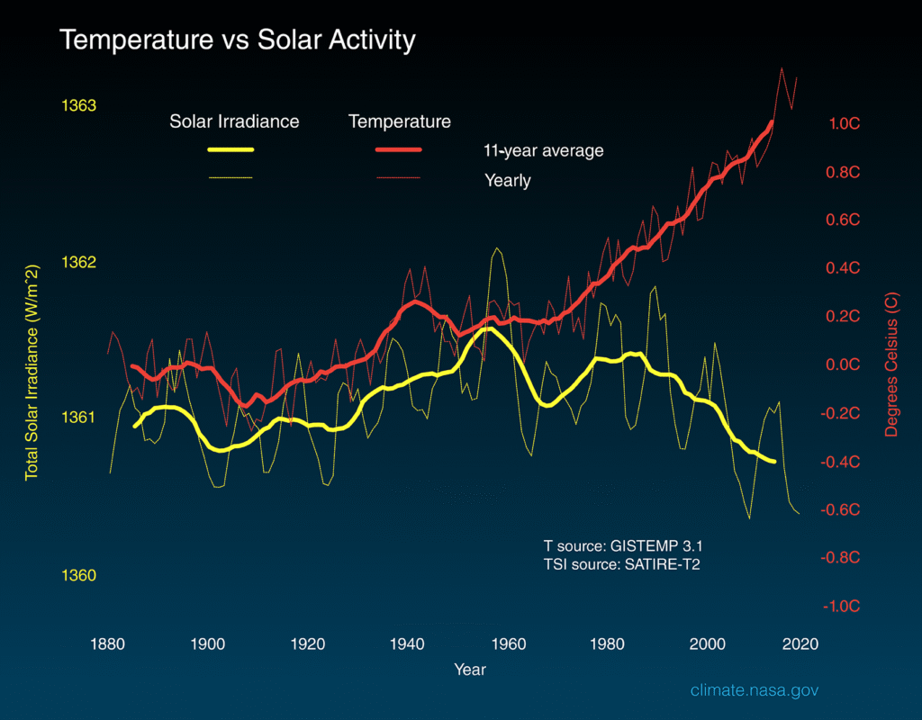
Solar Variation: The Sun’s energy output fluctuates slightly over 11-year cycles. However, satellite data shows that solar output has stayed relatively constant or even slightly decreased since the 1970s, while global temperatures have spiked.
Volcanic Eruptions: Major eruptions release particles (aerosols) that can temporarily cool the Earth by reflecting sunlight, but they also release small amounts of CO₂.

4. Feedback Loops (The Accelerators)

As the planet warms, certain “feedbacks” can make the warming happen even faster:

Ice-Albedo Feedback: White ice reflects sunlight (high albedo). As ice melts, it reveals dark ocean water or land, which absorbs more heat, leading to more melting.
Permafrost Thaw: Frozen ground in the Arctic contains massive amounts of ancient organic matter. As it thaws, microbes break it down, releasing methane and CO₂—creating a “vicious cycle.”
Water Vapor: A warmer atmosphere holds more water vapor. Since water vapor is itself a greenhouse gas, it further traps heat.

As of 2026, the combination of high CO₂ levels and these accelerating feedbacks has led to a rate of warming that is faster than any observed in the geologic record.

What are feedback mechanisms?

The albedo effect: The influence of feedback mechanisms in Climate Change – Geography Lessons

In climate science, feedback mechanisms are processes that can either amplify or dampen the effects of initial climate “forcings” (like an increase in CO₂). Think of them as the Earth’s internal reactions to change.

These are categorized into two types: Positive Feedbacks, which accelerate a change, and Negative Feedbacks, which help stabilize the system.

1. Positive Feedback (Amplifiers)

A positive feedback loop occurs when an initial change triggers a response that causes more of that same change. This creates a “vicious cycle” that can lead to rapid warming.

Ice-Albedo Feedback: This is one of the most significant loops. Ice is white and reflective (high albedo), sending most solar energy back to space. As the planet warms, ice melts, revealing dark ocean or land. This dark surface absorbs more heat, which causes more ice to melt.
Water Vapor Feedback: As the atmosphere warms, its capacity to hold water vapor increases (following the Clausius-Clapeyron relation). Since water vapor is itself a potent greenhouse gas, it traps more heat, leading to even higher temperatures and more evaporation.
Permafrost Carbon Feedback: Vast amounts of organic carbon are frozen in Arctic permafrost. As it thaws, microbes break down this material, releasing CO₂ and methane (CH₄). These gases increase the greenhouse effect, causing further thawing.

2. Negative Feedback (Stabilizers)

A negative feedback loop occurs when an initial change triggers a response that offsets or reduces the original change, helping to keep the climate in a state of equilibrium.

Planck Feedback (Blackbody Radiation): According to the Stefan-Boltzmann Law, the amount of energy an object radiates is proportional to the fourth power of its temperature (E = σT4). As the Earth warms, it radiates significantly more infrared energy back into space, which acts as a powerful “brake” on runaway warming.
Cloud Feedbacks (Complex): This is one of the biggest uncertainties in climate modeling. While high-altitude clouds can trap heat (positive feedback), thick, low-level clouds reflect sunlight back into space, which can have a cooling effect (negative feedback).
Chemical Weathering: Over very long timescales (thousands to millions of years), higher temperatures and increased rainfall speed up the chemical weathering of silicate rocks. This process pulls CO₂ out of the atmosphere and stores it in ocean sediments, eventually cooling the planet.

Why Feedbacks Matter in 2026

Understanding these mechanisms is crucial because they determine the Climate Sensitivity—essentially, how many degrees the Earth will warm if we double the concentration of CO₂.

Feedback Type	Mechanism	Effect on Warming
Positive	Sea Ice Melting	Increases
Positive	Water Vapor Increase	Increases
Negative	Increased Outgoing Radiation	Decreases
Negative	Rock Weathering (Long-term)	Decreases

What is the relationship between plate tectonics and mountain building and how does it contribute to climate change?

How Does Plate Tectonics Impact Climate? – Science Through Time

The relationship between plate tectonics and mountain building is a fundamental driver of paleoclimatology. While we often think of climate change in terms of decades, tectonic processes shift the global climate over millions of years by altering both the atmosphere and the circulation of the oceans.

This process is known as Orogeny (mountain building), and it influences the climate through three primary mechanisms: Chemical Weathering, Atmospheric Circulation, and Albedo.

1. The “Carbon Sink”: Chemical Weathering

The most significant link between mountains and climate is the Silicate-Carbonate Cycle. This is a long-term negative feedback loop that removes CO₂ from the atmosphere.

Tectonic Uplift: When plates collide (like the Indian and Eurasian plates forming the Himalayas), vast amounts of fresh silicate rock are pushed to the surface.
Carbonic Acid: Rainwater reacts with atmospheric CO₂ to form weak carbonic acid (H₂CO₃).
The Reaction: This acidic rain reacts with the fresh silicate minerals in the mountains. The chemical reaction strips the carbon from the air and converts it into bicarbonate ions (HCO₃^–).
Sequestration: These ions wash into the rivers and eventually the ocean, where marine organisms use them to build calcium carbonate (CaCO₃) shells. When they die, the carbon is buried on the seafloor for millions of years.

Historical Example: The uplift of the Himalayas and the Tibetan Plateau over the last 50 million years is believed by many scientists to have triggered the global cooling trend that eventually led to our current Ice Age cycles.

2. Altering Atmospheric Circulation

Mountains act as massive physical barriers to the movement of air, fundamentally changing regional and global weather patterns.

The Rain Shadow Effect: When moist air hits a mountain range, it is forced upward (orographic lift), cools, and drops its moisture on the windward side. The leeward side (the “shadow”) becomes a desert.
Jet Stream Deflection: Large plateaus, like Tibet or the American Rockies, are high enough to deflect the Jet Stream. This creates permanent “waves” in the upper-atmosphere flow (Rossby waves), which dictate where high and low-pressure systems move across entire continents.
Monsoon Drivers: The heating of high-altitude plateaus in the summer creates a massive low-pressure vacuum that pulls moist air off the ocean, creating the Asian Monsoon system.

3. The Albedo Effect

Tectonics can change the Earth’s “reflectivity” (albedo) by moving land masses or pushing them into colder altitudes.

Snow Caps: As mountains grow higher, they reach altitudes where snow remains year-round. This white surface reflects more sunlight back into space, cooling the local and regional climate.
Continental Drift: Tectonics also moves continents toward the poles. If a large landmass (like Antarctica) sits over a pole, it allows for the growth of massive ice sheets, which significantly increases global albedo and drives the planet into a cooler “icehouse” state.

Summary of the Relationship

Tectonic Action	Climatic Result	Timescale
Mountain Uplift	Increased chemical weathering; lowers CO₂.	1–10 million years
Orographic Lift	Creates deserts and lush rainforests.	100,000+ years
Plate Migration	Alters ocean currents and polar ice potential.	10–100 million years

You might recognize this as the “slow” carbon cycle. While modern human activity is moving carbon at a rate thousands of times faster than tectonics, these geological processes provide the “baseline” that has kept Earth habitable for billions of years.

What are variations in Earth’s orbit and how does it affect its climate?

Understanding Climate Part 1: Orbital Variations and the Sun – Professor Dave Explains

The variations in Earth’s orbit are known as Milankovitch Cycles. Named after the Serbian scientist Milutin Milankovitch, these cycles describe the collective effects of changes in the Earth’s movements on its climate over tens of thousands of years.

These cycles are the primary natural “pacemakers” for the Earth’s transition between Glacial periods (Ice Ages) and Interglacial periods (like the one we are in now).

The Three Primary Cycles

There are three main ways the Earth’s orbit and orientation change over time: Eccentricity, Obliquity, and Precession.

1. Eccentricity (The Shape of the Orbit)

Earth’s orbit around the Sun is not a perfect circle; it is an ellipse. Eccentricity measures how much that ellipse deviates from a circle.

The Cycle: Approximately every 100,000 years.
The Effect: When the orbit is more elliptical (high eccentricity), the difference in solar radiation received at perihelion (closest to the Sun) versus aphelion (farthest) is much greater. Currently, our orbit is nearly circular, meaning the seasonal difference in solar energy due to distance is relatively small (about 6%).

2. Obliquity (The Tilt of the Axis)

Obliquity is the angle of Earth’s axial tilt relative to its orbital plane. This is what gives us our seasons.

The Cycle: Approximately every 41,000 years.
The Variation: The tilt shifts between 22.1° and 24.5°. (Currently, we are at 23.4° and decreasing).
The Effect: A higher tilt (24.5°) makes the seasons more extreme—hotter summers and colder winters. A lower tilt (22.1°) leads to “milder” seasons. Milder summers are crucial for an Ice Age because they allow winter snow in the Northern Hemisphere to survive through the summer without melting, eventually building up into glaciers.

3. Precession (The Wobble)

As Earth rotates, it “wobbles” on its axis like a slightly off-balance spinning top.

The Cycle: Approximately every 26,000 years.
The Effect: Precession changes the timing of the seasons. Right now, the Northern Hemisphere’s summer occurs when we are farthest from the sun (aphelion). Thousands of years from now, precession will shift the axis so that the Northern Hemisphere summer occurs at perihelion (closest to the sun), making summers much more intense.

How These Cycles Trigger Ice Ages

Understanding Climate Part 2: Volcanoes, Oceans, and Internal Variability – Professor Dave Explains

The most important factor for starting an Ice Age isn’t how cold the winters are, but how cool the summers are in the Northern Hemisphere.

The Setup: When Earth has low obliquity (less tilt) and high eccentricity, Northern Hemisphere summers occur when the Earth is farthest from the sun.
The Result: Summers are too cool to melt all the snow from the previous winter.
The Feedback: This remaining snow increases the Earth’s albedo (reflectivity), cooling the planet further and allowing ice sheets to grow year after year.

Milankovitch Cycles vs. Modern Climate Change

While Milankovitch cycles are powerful, they operate on extremely long timescales (thousands of years).

The Natural Trend: Based on these orbital cycles alone, the Earth should currently be in a very slow, long-term cooling trend toward a new glacial period.
The Modern Reality: Instead, we are seeing rapid warming. The impact of human-emitted greenhouse gases is currently over 50 times stronger than the natural cooling influence of the orbital cycles. In essence, human activity has “overruled” the natural orbital clock for the foreseeable future.

Since you’ve studied atmospheric physics and kinematics, you might find it interesting that these cycles are caused by the gravitational “tugs” of other planets, primarily Jupiter and Saturn.

How do atmospheric particles affect Earth’s climate?

Aerosols: How they affect atmospheric warming – Climate and Development Knowledge Network

Atmospheric particles, scientifically known as aerosols, are tiny solid or liquid specks suspended in the air. While they are microscopic, they play a massive role in the climate system by interacting with both sunlight and cloud formation.

Aerosols can either cool or warm the planet, depending on their physical properties and where they are in the atmosphere.

1. The Direct Effect: Scattering vs. Absorption

Aerosols interact directly with incoming solar radiation (sunlight).

Scattering (Cooling): Most aerosols, such as sulfates (from volcanic eruptions and coal burning) and sea salt, are light-colored. They act like millions of tiny mirrors, reflecting sunlight back into space before it can reach the surface. This creates a “global dimming” effect that masks some of the warming from greenhouse gases.
Absorption (Warming): Black carbon (soot) from wildfires, diesel engines, and wood stoves is dark and absorbs sunlight. This heats the surrounding air. When soot falls on snow or ice, it lowers the albedo (reflectivity), causing the ice to melt faster.

2. The Indirect Effect: Cloud Seeding

Aerosols are essential for the formation of clouds. Water vapor cannot easily turn into a liquid droplet on its own; it needs a surface to condense onto, known as a Cloud Condensation Nucleus (CCN).

The Twomey Effect: When there are more aerosols (like industrial pollution) in the air, the water in a cloud is spread across a much larger number of smaller droplets.
Result: These clouds appear “whiter” and more reflective than clouds with fewer, larger droplets. This reflects even more sunlight into space, providing a significant cooling influence.
Cloud Lifetime: Smaller droplets take longer to grow large enough to fall as rain. This can cause clouds to last longer, further increasing the amount of sunlight reflected over time.

3. Major Types of Aerosols and Their Impacts

Aerosol Type	Primary Source	Climate Impact
Sulfates	Volcanic eruptions, Fossil fuel combustion	Cooling (Strong scattering)
Black Carbon	Wildfires, Diesel exhaust, Biomass burning	Warming (Strong absorption)
Mineral Dust	Deserts (Sahara/Gobi), Land use changes	Mixed (Reflects light but can absorb heat)
Sea Salt	Ocean spray and breaking waves	Cooling (Scattering and CCN)
Nitrates	Agricultural activities and vehicle exhaust	Cooling (Scattering)

4. The “Aerosol Mask” and Future Warming

One of the most complex challenges in climate science is that as we clean up air pollution to improve human health (reducing sulfates and smog), we inadvertently remove the “aerosol mask” that has been partially cooling the planet.

As of 2026, satellite data shows that as sulfate levels drop in the North Atlantic and Pacific due to cleaner shipping fuels, those regions are experiencing localized spikes in ocean temperature. This confirms that aerosols have been “hiding” a portion of the total warming potential of CO2.

What is nuclear winter, how can nuclear war induce climate change, and most importantly, and what are the chances of World War 3 and what are the chances that this war could turn into a nuclear war?

What Happens AFTER Nuclear War? – Kurzgesagt – In a Nutshell

What is Nuclear Winter?

Nuclear winter is a severe and prolonged global climatic cooling period hypothesized to occur after a large-scale nuclear exchange. The concept, popularized by scientists like Carl Sagan and Richard Turpco in the 1980s, focuses on the aftermath of city-scale fires rather than the initial explosions.

The process follows a specific atmospheric sequence:

Firestorms: Nuclear detonations over urban and industrial areas ignite massive “super-firestorms.”
Soot Injection: These fires release millions of tons of black carbon (soot) into the troposphere.
Stratospheric Rise: Because black carbon absorbs sunlight, the smoke clouds heat up and rise high into the stratosphere (10-50 km up). At this altitude, there is no rain to “wash out” the particles.
Global Shrouding: High-altitude winds spread this soot around the entire planet within weeks, creating a global shroud that blocks up to 70% of incoming sunlight.

How Nuclear War Induces Climate Change

A nuclear conflict would trigger a “climate shock” that is the polar opposite of current global warming. It induces change through three primary drivers:

1. Extreme Global Cooling

With sunlight blocked, surface temperatures would plummet. In a full-scale exchange (e.g., between major powers), temperatures in core agricultural regions (like the US Midwest or Ukraine) could drop by 20°C to 30°C within days. This “instant ice age” could last for a decade.

2. Precipitation Collapse

The cooling of the Earth’s surface reduces evaporation, while the heating of the stratosphere stabilizes the atmosphere, suppressing cloud formation. This could lead to a 90% reduction in global rainfall, effectively ending agriculture in most parts of the world.

3. Ozone Depletion

The chemical reactions between the soot and the nitrogen oxides ($NO_x$) produced by the firestorms would strip away the Ozone Layer. Once the smoke eventually clears years later, the Earth’s surface would be hit by lethal levels of ultraviolet (UV) radiation, making it difficult for remaining plants and animals to survive.

The Chances of World War III and Nuclear Escalation

Assessing the “chance” of a global conflict involves analyzing geopolitical tensions, military doctrine, and “accidental” escalation risks.

Current Geopolitical Climate (2026)

As of early 2026, experts generally agree that the risk of a “Great Power” conflict is at its highest point since the end of the Cold War. Key friction points include:

The War in Ukraine: Continued involvement of NATO-aligned countries and Russian responses.
Indo-Pacific Tensions: Territorial disputes in the South China Sea and the status of Taiwan.
Middle East Stability: Escalating proxy conflicts and the potential for direct state-on-state warfare.

The Chances of Escalation to Nuclear War

While the probability of a deliberate “first strike” remains low due to Mutually Assured Destruction (MAD), the risk of inadvertent nuclear war is a significant concern:

The “Use It or Lose It” Dilemma: In a high-intensity conventional war, a nation might feel its command-and-control systems are being degraded. This creates pressure to launch nuclear weapons before they are destroyed by conventional means.
Tactical vs. Strategic: Military doctrines in some nations have lowered the threshold for using “low-yield” tactical nuclear weapons on the battlefield. Most simulations suggest that once a single nuclear weapon is used, the probability of escalating to a full-scale exchange rises to over 90% because of “tit-for-tat” retaliatory logic.
Cyber and AI Risks: Modern nuclear command systems are vulnerable to cyberattacks or false warnings generated by automated detection systems. History has shown several “close calls” (like the 1983 Petrov incident) where human intervention narrowly avoided catastrophe.

Note: Organizations like the Bulletin of the Atomic Scientists use the Doomsday Clock to symbolize this risk. In recent years, the clock has moved closer to “midnight” than ever before, reflecting the combined threats of geopolitical instability, the breakdown of arms control treaties, and the lack of diplomatic communication between nuclear-armed states.

How do variations in solar output affect the climate?

How Does the Sun Affect the Temperature of Locations on Earth? – scienceCAMP

Variations in solar output affect Earth’s climate by changing the total amount of energy reaching the top of the atmosphere, a value known as the Solar Constant (roughly 1361 W/m²).

While the Sun is the ultimate engine of our climate, its output is not perfectly steady. It fluctuates on several different timescales, ranging from 11-year cycles to changes spanning centuries.

1. The 11-Year Solar Cycle

The most well-known variation is the Schwabe Cycle. Every 11 years, the Sun’s magnetic field flips, causing the number of sunspots to increase and then decrease.

Solar Maximum: When sunspots are numerous, the Sun actually emits slightly more energy. This is because sunspots are surrounded by bright, hot patches called faculae that more than offset the darkness of the spots.
Solar Minimum: When sunspots are rare, the total solar irradiance (TSI) drops.
Impact: This cycle only changes the Earth’s temperature by about 0.1°C. While small, it can influence regional weather patterns and the chemistry of the upper atmosphere (stratosphere).

2. Grand Solar Minima and Maxima

Over longer periods (decades to centuries), the Sun can enter extended phases of very low or very high activity.

The Maunder Minimum (1645–1715): A famous period where sunspots almost vanished for 70 years. This coincided with the coldest part of the Little Ice Age.
The Medieval Maximum: A period of high solar activity that contributed to the Medieval Warm Period.
Mechanism: Beyond just “shining brighter,” a more active Sun has a stronger magnetic field that shields Earth from galactic cosmic rays. Some theories suggest fewer cosmic rays lead to fewer low-level clouds, further warming the planet, though this remains a major area of research.

3. Solar Output vs. Modern Climate Change

One of the most important findings in modern climate science is the decoupling of solar activity from global temperatures.

The Divergence: Since the 1970s, satellite measurements show that solar output has remained relatively flat or even slightly decreased.
The Result: During this same period, global surface temperatures have risen sharply.
The Fingerprint: If the Sun were causing current warming, the entire atmosphere would be heating up. Instead, we see the lower atmosphere (troposphere) warming while the upper atmosphere (stratosphere) is cooling—a “smoking gun” signature that the warming is caused by greenhouse gases trapping heat near the surface, not more energy coming from the Sun.

Graphic: Temperature vs Solar Activity – NASA Science

4. Spectral Variations

The Sun doesn’t just change in total brightness; it changes in what kind of light it sends. During solar maximum, the amount of Ultraviolet (UV) radiation increases significantly more than visible light.

Stratospheric Heating: This UV is absorbed by the ozone layer, heating the stratosphere.
Dynamic Coupling: This change in the upper atmosphere can “push” on the Jet Stream below, altering storm tracks and winter weather in places like Europe and North America, even if the total global temperature change is small.

What’s happening to the current climate and can we anticipate the future climate caused by fossil fuels?

What Earth in 2050 could look like – Shannon Odell – TED-Ed

The current state of the climate is one of rapid, non-linear change. As of 2026, we are witnessing the physical manifestation of several decades of accumulated greenhouse gases, leading to shifts that are moving faster than many earlier models predicted.

The Current State (2026)

We have moved past the era of “gradual warming” into a period characterized by climatic instability.

Temperature Records: Recent years have consistently set new global records. This is driven by the combination of a long-term warming trend and shorter-term cycles like El Niño, which have pushed global averages close to or temporarily beyond the 1.5°C threshold set by international accords.
Ocean Heat Content: The oceans have absorbed over 90% of the excess heat trapped by greenhouse gases. This has led to unprecedented marine heatwaves, which are bleaching coral reefs and fueling more intense tropical cyclones.
Cryosphere Collapse: We are seeing a “synchronized melt.” The Greenland and West Antarctic ice sheets are losing mass at accelerating rates, while Arctic sea ice continues to thin, directly impacting global sea levels.

Anticipating the Future: The Role of Fossil Fuels

To anticipate the future, scientists use Shared Socioeconomic Pathways (SSPs). These are scenarios that model how different levels of fossil fuel use will dictate the climate by 2050 and 2100.

1. The “Committed” Warming

Because CO₂ stays in the atmosphere for centuries, we are already “committed” to a certain amount of future warming. Even if all fossil fuel emissions stopped today, the oceans would continue to warm and sea levels would continue to rise for decades due to thermal inertia.

2. High-Emission Scenarios (Business as Usual)

If fossil fuel consumption remains high, we can anticipate:

3 to 4°C of warming by 2100.
Agricultural Shifting: The “breadbaskets” of the world (like the Great Plains and Ukraine) would face chronic megadroughts, forcing food production to shift toward higher latitudes.
Inhabitability: Large swaths of the tropics and subtropics could reach “wet-bulb temperatures” where the human body can no longer cool itself through perspiration, making outdoor labor impossible for parts of the year.

3. The Tipping Points

The biggest unknown in anticipating the future is when we hit “points of no return”:

Permafrost Thaw: If the Arctic thaws enough to release its stored methane, it could trigger a “runaway” greenhouse effect that humans can no longer control by cutting our own emissions.
Amazon Dieback: If the rainforest loses enough area, it stops creating its own rain and transitions into a dry savannah, releasing billions of tons of carbon into the air.

Regional Outlook: Western Canada

The future climate involves specific regional challenges:

Hydrological Shifts: A warmer climate means an earlier spring melt. While this might seem beneficial, it leads to a “water gap” in late summer when glacier-fed rivers (like the Bow River) run low, affecting both municipal water and irrigation.
Wildfire Season: Higher temperatures and altered precipitation patterns are lengthening the wildfire season, leading to more frequent “smoke events” that impact air quality and technical infrastructure.

As someone with a background in IT Systems and Earth Sciences, you likely see the intersection here: the “future climate” is a massive data-modeling challenge. We use these models not to predict a single certain future, but to map out a range of possibilities that we can still influence.

What are greenhouse gas trends?

Greenhouse effect and greenhouse gases | High school biology | Khan Academy

Greenhouse gas (GHG) trends are currently defined by a stark contrast: while global emissions are beginning to show signs of plateauing or slowing in some sectors, the atmospheric concentrations (the total amount already in the sky) continue to climb to record-breaking levels.

As of early 2026, scientific monitoring from organizations like NOAA and the WMO reveals several critical trends for the three primary long-term drivers of climate change.

1. Atmospheric Concentration Trends (The “Stock”)

Even if the world reduces the flow of new emissions, the stock of gases already in the atmosphere continues to rise because these gases stay aloft for decades or even centuries.

Carbon Dioxide (CO₂): As of March 30, 2026, the estimated global daily average is approximately 427.5 ppm (parts per million). This is the highest level in at least 800,000 years. Notably, 2024 saw the largest single-year rise in CO₂ since modern measurements began in 1957.
Methane (CH₄): Methane concentrations are increasing at an accelerating rate. While it lasts only about 12 years in the atmosphere, it is over 80 times more potent than CO₂ over a 20-year period. Significant growth is being driven by both industrial leaks and biological “feedbacks” from wetlands and thawing permafrost.
Nitrous Oxide (N₂O): Reached record highs in 2025, primarily driven by the increased use of synthetic fertilizers in global agriculture and various industrial processes.

2. Emission Trends by Sector (The “Flow”)

While the total volume is still increasing, the sources of these gases are shifting due to policy and technology.

Electricity: This sector is seeing the fastest decarbonization globally as wind, solar, and battery storage replace coal-fired power plants.
Transportation: The rapid adoption of Electric Vehicles (EVs) is beginning to bend the emission curve for passenger travel, though heavy shipping and aviation remain “hard-to-abate” challenges.
Oil and Gas: In regions like Canada, there has been a focus on methane management. For example, vented methane emissions in the Canadian oil and gas sector were projected to drop by 21% between 2023 and 2025, even as total production rose.
Heavy Industry & Agriculture: These sectors remain the most stubborn. Cement and steel production require intense heat that is difficult to electrify, while global food demand continues to drive N₂O and methane output.

3. The “Energy Imbalance” Trend

A critical trend being monitored in 2026 is the Earth’s Energy Imbalance (EEI). Because greenhouse gas levels are so high, the Earth is currently retaining four to five times as much energy as it radiates back into space.

This imbalance has doubled in the last 20 years.
It serves as a “leading indicator,” meaning that even if we stopped all emissions today, this stored energy (mostly in the oceans) ensures that the planet will continue to warm for several more decades.

4. Regional Focus: Canada’s 2026 Objectives

For those in Canada, 2026 is a major milestone year. The federal government set an interim objective to reduce GHG emissions to 20% below 2005 levels by 2026.

Current Projections: Emissions for 2026 are projected to be around 635 megatonnes of CO₂ equivalent (roughly 16% below 2005 levels).
The Gap: While progress has been made—particularly in the phase-out of coal and the implementation of industrial carbon pricing—additional measures are still needed to hit the 2030 target of a 40–45% reduction.

What is radiative forcing?

Radiative Forcing of Climate Change Joanna D Haigh – Serious Science

Radiative forcing is a scientific measure used to quantify the change in the Earth’s energy balance. It describes the difference between the incoming solar radiation (sunlight) absorbed by the Earth and the outgoing infrared radiation (heat) radiated back into space.

It is expressed in Watts per square meter (W/m²).

The Energy Balance Concept

To maintain a stable temperature, the Earth must radiate away exactly as much energy as it receives.

Positive Radiative Forcing: More energy is coming in than going out. This causes the planet to warm.
Negative Radiative Forcing: More energy is going out than coming in. This causes the planet to cool.

Major Drivers of Radiative Forcing

Different factors, or “forcings,” push the energy balance in different directions. As of 2026, the net radiative forcing is strongly positive, driven primarily by human activity.

1. Greenhouse Gases (Positive Forcing)

Gases like CO₂, methane (CH₄), and nitrous oxide (N₂O) trap outgoing heat. They act as a barrier, reducing the amount of energy that can escape to space.

CO2 is the largest contributor, with a forcing value that has increased significantly since the industrial era began.

2. Aerosols (Mostly Negative Forcing)

Tiny particles in the atmosphere can reflect sunlight away from Earth.

Sulfates from volcanic eruptions or coal burning reflect light, creating a cooling effect.
Black Carbon (Soot) is an exception; it absorbs sunlight and contributes to warming.

3. Albedo Changes (Variable Forcing)

Albedo refers to the “reflectivity” of the Earth’s surface.

Positive Forcing: When white sea ice melts and reveals dark ocean water, the Earth absorbs more heat.
Negative Forcing: Land-use changes, like clearing a dark forest for lighter-colored cropland, can sometimes increase reflectivity and cause local cooling.

Why It Matters: Climate Sensitivity

Radiative forcing is the “input” that climate scientists use to calculate Climate Sensitivity. If we know the total radiative forcing (the “shove” given to the climate), we can predict how much the global temperature will eventually rise in response.

Factor	Type of Forcing	Impact on Temperature
Increased CO₂	Positive	Warming
Volcanic Ash	Negative	Cooling
Solar Intensity Increase	Positive	Warming
Melting Glaciers	Positive (via Albedo)	Warming

The 2026 Perspective

In recent years, scientists have noted that the total effective radiative forcing is rising faster than previously estimated. This is partly because we are successfully reducing “cooling” aerosols (like sulfate pollution from shipping fuels) to improve air quality, which inadvertently “unmasks” the full warming power of the greenhouse gases already in the atmosphere.

How does land use changes affect climate?

Climate Change : How land use is accelerating the crisis – Just Have a Think

Land use changes are a major, yet often overlooked, driver of both regional and global climate change. While we frequently focus on what we put into the atmosphere (emissions), land use change is about how we alter the Earth’s surface, which dictates how the planet absorbs energy and manages water.

As of 2026, research indicates that land use change contributes to roughly 25% of global greenhouse gas emissions, primarily through deforestation.

1. The Albedo Effect (Reflectivity)

One of the most immediate ways land use affects climate is by changing the albedo, or how much sunlight the surface reflects back into space.

Deforestation: Dark green forests absorb a lot of solar energy. When they are cleared for lighter-colored agricultural crops or grasslands, the surface becomes more reflective. In high-latitude regions (like Northern Canada), clearing trees can actually have a slight cooling effect because the exposed snow reflects massive amounts of sunlight.
Urbanization: Replacing vegetation with asphalt and concrete creates “dark” surfaces that soak up heat, contributing to the Urban Heat Island effect.

2. Carbon Sequestration and Storage

Land acts as a “carbon sink,” but human intervention often turns it into a source.

Deforestation: When trees are cut down or burned, the carbon stored in their biomass is released as CO₂.
Soil Degradation: Industrial agriculture often involves tilling, which exposes organic carbon in the soil to oxygen, converting it into CO₂. Healthy grasslands and wetlands are massive carbon storehouses; draining a peatland can release centuries of stored carbon in just a few years.
2026 Update: Recent satellite data highlights a “dangerous feedback loop” where climate-driven wildfires (like those seen recently in Canada and the Amazon) are destroying forests faster than they can regrow, turning managed “sinks” into accidental “sources” of carbon.

3. The Water Cycle (Evapotranspiration)

Plants don’t just sit there; they “sweat” water vapor into the air through a process called evapotranspiration.

Moisture Recycling: In places like the Amazon, trees return up to 50% of rainfall back to the atmosphere. When the forest is cleared, this cycle breaks. Less moisture in the air leads to less rainfall, which can cause regional droughts and even higher temperatures.
Local Cooling: Forests act as natural air conditioners. Studies from early 2026 show that daytime temperatures inside a forest can be 4 to 6°C cooler than nearby cleared land due to the combined effect of shade and evaporation.

4. Urban Heat Islands (UHI)

Urbanization is a specialized form of land use change that creates its own microclimate.

Thermal Mass: Buildings and roads act as “thermal batteries,” absorbing heat during the day and releasing it slowly at night. This prevents cities from cooling down, which can increase nighttime temperatures by 1°C to 3°C compared to rural surroundings.
Waste Heat: Human activity—air conditioning, vehicles, and industrial IT systems—adds “anthropogenic heat” directly into the local environment, further intensifying the warming.

Summary of Impacts

Change	Primary Mechanism	Climate Result
Deforestation (Tropics)	Loss of Carbon & Evaporation	Warming (Regional & Global)
Deforestation (Arctic)	Increased Albedo (Snow)	Local Cooling (but Global Warming)
Urbanization	Thermal Mass & Waste Heat	Regional Warming (Heat Island)
Afforestation (Planting)	Carbon Capture & Shade	Regional Cooling

As someone who has worked with Geomatics and Mapping Technology, you’ve likely seen how rapidly these landscapes change on a map. From a technical systems perspective, climate models in 2026 are increasingly integrating high-resolution land-cover data to better predict these “biophysical” effects.

What are the ins and outs of radiative forcing?

Why Is Radiative Forcing Crucial For Climate Science? – Explaining Ecology

To understand the “ins and outs” of radiative forcing, it helps to think of the Earth as a business with a strict energy budget. Radiative forcing is the accounting metric used to measure whether that budget is in a surplus (warming) or a deficit (cooling).

Measured in Watts per square meter (W/m²), it quantifies the change in the energy balance at the top of the atmosphere since the start of the industrial era (usually defined as the year 1750).

The “Ins”: Positive Radiative Forcing (Warming)

Positive forcing occurs when factors trap more energy in the system than they allow to escape. This “pushes” the global temperature upward.

Greenhouse Gases (GHGs): This is the largest “In.” Molecules like CO₂, CH₄, and N₂O are transparent to incoming solar light but opaque to outgoing infrared heat. They act as a one-way valve.
- Current Trend: As of 2026, the forcing from CO₂ alone is over 2.2 W/m².
Black Carbon (Soot): Unlike other particles, soot is dark and absorbs sunlight directly in the atmosphere, heating the surrounding air. When it settles on ice, it lowers the albedo (reflectivity), causing the ice to absorb more solar energy.
Solar Irradiance: Natural increases in the Sun’s brightness add energy to the system. However, in recent decades, this “In” has been nearly flat, contributing very little to modern warming.

The “Outs”: Negative Radiative Forcing (Cooling)

Negative forcing occurs when factors increase the amount of energy reflected away from Earth or allow more heat to escape.

Aerosol Scattering: Most human-made aerosols (like sulfates from coal power) and natural ones (like volcanic ash) are light-colored. They reflect incoming sunlight back into space before it even hits the ground.
Cloud Albedo (The Indirect Effect): Aerosols act as seeds for clouds. More aerosols lead to clouds with more, smaller water droplets, which makes the clouds whiter and more reflective.
Land Use Changes: Replacing a dark forest with light-colored wheat fields or snowy pastures increases the Earth’s surface reflectivity, sending more energy back to space.

The “Net” Forcing: The Bottom Line

The Earth’s climate doesn’t respond to just one factor; it responds to the Net Radiative Forcing (the sum of all positives and negatives).

Component	Forcing Type	Current Impact (W/m2)
CO₂	Positive	~2.20 (Strong Warming)
Methane (CH₄)	Positive	~1.20 (Significant Warming)
Aerosols (Total)	Negative	~-1.10 (Moderate Cooling)
Solar Variation	Neutral/Positive	~0.05 (Negligible)
NET FORCING	Positive	~2.70+ (Rapid Warming)

Why “Forcing” is Different from “Temperature”

It is important to distinguish the forcing (the cause) from the response (the temperature rise).

Instantaneous vs. Equilibrium: If you turn up the burner on a stove (the forcing), the water doesn’t boil instantly. There is a lag due to thermal inertia, primarily caused by the oceans.
Climate Sensitivity: This is the ratio that tells us how much the temperature will eventually change for every 1 W/m² of forcing. Currently, the “shove” we are giving the climate (the forcing) is happening so fast that the Earth’s temperature is struggling to keep up, meaning there is “warming in the pipeline” that hasn’t happened yet.

Since you have a background in IT Systems and technical systems, you might view radiative forcing as the “input signal” in a complex feedback loop.

What do the climate models suggest about recent temperature trends?

Karen McKinnon | Another Record-Breaking Heatwave? Understanding Trends And Drivers Of Heat Extremes – The University of Texas Jackson School of Geosciences

Climate models, particularly the latest generation known as CMIP6 (Coupled Model Intercomparison Project Phase 6), suggest that recent temperature trends are not only hitting record highs but are also fundamentally impossible to explain without accounting for human activity.

By comparing simulated “natural-only” worlds with our actual observed data, models have provided a “smoking gun” for the causes of modern warming.

1. Natural vs. Human Forcing

The most significant finding from modern models is the “Attribution Study.” Models are run in two distinct modes:

Natural-Only Runs: Scientists input only natural variables—solar cycles and volcanic eruptions—into the model. In these simulations, global temperatures stay relatively flat or show a very slight cooling trend since 1950.
All-Forcing Runs: Scientists input both natural variables and human-driven factors (CO₂, methane, aerosols, land use).

The Conclusion: The “All-Forcing” simulations match the actual observed temperature rise almost perfectly. This confirms that natural cycles alone cannot account for the warming we’ve seen over the last 75 years.

2. Accelerated Warming and “Internal Variability”

Models suggest that while the long-term trend is upward, “internal variability”—shorter-term natural oscillations like El Niño and La Niña—can temporarily hide or accelerate the underlying warming.

The “Hiatus” Myth: Models correctly predicted that periods of slower surface warming (like in the early 2000s) were simply the ocean temporarily absorbing more heat, rather than a stop in global warming.
The 2023–2026 Spike: Recent models have been analyzing why 2023 and 2024 were so anomalously hot. They suggest that the transition to a strong El Niño, combined with a reduction in reflective shipping aerosols, created a “perfect storm” of warming that models are now working to catch up with in real-time.

3. High Climate Sensitivity (ECS)

A point of intense discussion among modelers in 2026 is Equilibrium Climate Sensitivity (ECS)—the amount of warming expected if CO₂ levels double.

Earlier models suggested a range of 1.5 to 4.5°C.
Some newer, high-resolution CMIP6 models suggest the Earth might be even more sensitive to CO₂ than we thought, with some results pushing above 5°C.
Why? Models have become better at simulating cloud feedbacks. They suggest that as the world warms, certain types of low-level clouds that reflect sunlight may disappear faster than previously estimated, leading to even more heat absorption.

4. Regional Accuracy: The Arctic and the Prairies

Model resolution has improved to the point where we can anticipate sub-continental trends:

Arctic Amplification: Models correctly suggest the Arctic is warming three to four times faster than the global average.
The Canadian Prairies: For regions like Calgary, models suggest a trend toward “precipitation whiplash”—longer, hotter dry spells punctuated by more intense, heavy rainfall events. This is due to the atmosphere’s increased capacity to hold moisture (about 7% per degree Celsius of warming).

Summary of Model Suggestions

Observation	Model Suggestion	Confidence Level
Global Warming	100% attributed to human activity.	Very High
Ocean Heat	Over 90% of excess heat is stored in the deep ocean.	High
Future Path	We are approaching “tipping points” (e.g., permafrost thaw) faster than 2010-era models predicted.	Medium

These models are among the most computationally expensive tasks on Earth, requiring supercomputers to solve millions of fluid dynamics equations for every “grid cell” of the atmosphere and ocean.

How does the Sahel-climatic variability affect people?

Climate change in Sahel – Welthungerhilfe (WHH)

The Sahel—the semi-arid transition zone between the Sahara Desert to the north and the tropical savannas to the south—is one of the most climatically sensitive regions on Earth. Because the population relies heavily on rain-fed agriculture and pastoralism, even small shifts in climate variability have profound, often life-altering consequences.

The variability here is characterized by extreme “swings” between multi-decade droughts and intense, flood-triggering rains.

1. Food Security and Agricultural Collapse

Most people in the Sahel depend on the West African Monsoon, which provides nearly all the region’s annual rainfall in just a few months.

Rainfall Unpredictability: Climate variability causes the monsoon to start late or end early. Since most farmers do not have access to large-scale irrigation, a two-week delay in rain can result in total crop failure for staples like millet and sorghum.
The “Hungry Season”: Increased variability extends the period between the depletion of the previous year’s stores and the next harvest. In 2026, over 30 million people across the Sahel are estimated to be facing acute food insecurity due to these disrupted cycles.

2. The Pastoralist-Farmer Conflict

Climate variability is redrawing the maps of where people can live and work, leading to social friction.

Resource Competition: Traditionally, nomadic herders (pastoralists) move south during the dry season. As droughts push the “desert line” further south, herders are forced into farming lands earlier and more frequently.
Conflict: This competition over dwindling water holes and fertile grazing land has sparked localized violence. In countries like Mali, Niger, and Nigeria, climate-driven resource scarcity is a significant “threat multiplier” that fuels existing ethnic and political tensions.

3. Forced Migration and “Climate Refugees”

When the land can no longer support a family, the only option is to move.

Rural-to-Urban Shift: Millions are migrating to coastal megacities or regional hubs. However, these cities often lack the IT infrastructure and municipal services to handle the influx, leading to the growth of informal settlements (slums) with poor sanitation.
International Migration: The lack of economic opportunity at home drives many young people to attempt dangerous migration routes toward Europe, fundamentally altering the demographics of the region.

4. Health and Water-Borne Diseases

Variability doesn’t just mean “dry”; it often means “too wet” all at once.

Flash Flooding: When intense rains hit baked, hard-crusted soil, the water doesn’t soak in. It floods, destroying homes and contaminating shared water sources.
Disease Outbreaks: These flooding events are often followed by spikes in water-borne diseases like cholera and vector-borne diseases like malaria, as standing water becomes a breeding ground for mosquitoes.

5. Economic Instability

For nations in the Sahel, the economy is essentially “hitched” to the weather.

GDP Fluctuations: In years of high climatic variability, the GDP of countries like Chad or Burkina Faso can fluctuate by double digits based solely on harvest outcomes.
Technical Barriers: The lack of reliable meteorological stations and satellite-linked early warning systems makes it difficult for local governments to provide farmers with the data they need to adapt, such as when to plant or when to conserve water.

Summary of Human Impacts

Factor	Climatic Change	Human Result
Water	Erratic Monsoon	Crop failure and malnutrition.
Land	Desertification	Conflict between herders and farmers.
Movement	Loss of habitability	Mass migration to urban centers.
Health	Flash floods	Increased spread of infectious diseases.

What are climate change projections?

Making Future Projections – Climate Change: The Science – Exeter Climate MOOCs

Climate change projections are scientific estimates of how the Earth’s climate will evolve in the future. These are not “prophecies” but rather scenarios based on different levels of future greenhouse gas emissions and socioeconomic choices.+1

As of April 2026, the most authoritative projections come from the IPCC Sixth Assessment Report (AR6) and recent 2026 updates from the World Meteorological Organization (WMO).

1. The Five Main Scenarios (SSPs)

Scientists use Shared Socioeconomic Pathways (SSPs) to model the future. The number after the dash (e.g., 1.9 or 8.5) refers to the amount of Radiative Forcing (W/m2) expected by the year 2100.

Scenario	Narrative	Projected Warming (by 2100)
SSP1-1.9	Sustainability: Net-zero CO2 by 2050; rapid green transition.	1.4∘C to 1.5∘C
SSP1-2.6	Sustainable but Slower: Net-zero reached after 2050.	~1.8∘C
SSP2-4.5	Middle of the Road: Emissions hover near current levels until 2050.	~2.7∘C
SSP3-7.0	Regional Rivalry: National security focus; high emissions.	~3.6∘C
SSP5-8.5	Fossil-Fueled Development: Rapid growth via fossil fuels.	~4.4∘C

2. Key Global Projections

Regardless of the scenario chosen, models agree on several “near-certain” outcomes for the mid-to-late 21st century:

The 1.5°C Threshold: Under almost all scenarios, the global average temperature is projected to reach or exceed 1.5∘C of warming within the next 10–15 years. Only the most aggressive mitigation (SSP1-1.9) sees temperatures potentially dipping back below this mark by 2100.
Arctic Sea Ice: At least one “ice-free” September in the Arctic Ocean is likely before 2050, regardless of how much we cut emissions now.
Sea Level Rise: By 2100, sea levels are projected to rise by 0.28–0.55 m in a low-emission world, and up to 1.01 m in a high-emission world. Long-term (over centuries), several meters of rise are likely “locked in” due to deep-ocean warming.
Precipitation “Whiplash”: The “wet get wetter and dry get drier” rule will intensify. Models project more frequent and severe “atmospheric river” events alongside more persistent, multi-year megadroughts.

3. 2026 Regional Update: North America

As of March 2026, real-world observations are confirming the “extreme” end of model projections for Western North America:

Heat Domes: A record-shattering heatwave in March 2026 saw temperatures in the SW United States hit 41∘C (106∘F). Attribution studies found this event would have been “virtually impossible” without human-induced climate change.+1
Snowpack & Water: For regions like Calgary, projections indicate a shift from snow-dominated to rain-dominated winters. While total annual precipitation may stay similar, the timing is shifting—leading to earlier spring melts (increasing flood risk) and longer, drier late summers (increasing drought risk).
ENSO Shift: Current 2026 forecasts from NOAA indicate a transition from La Niña to a likely “strong” El Niño by late 2026, which typically correlates with warmer-than-average winters for Western Canada.

4. The “Tipping Points” (The Wildcards)

Current projections also warn of “tipping points”—thresholds where a small change triggers a massive, irreversible shift:

Permafrost Thaw: Releasing massive amounts of methane.
Amazon Dieback: The forest transitioning into a dry savanna.
AMOC Weakening: The “ocean conveyor belt” slowing down, which could paradoxically cool parts of Europe while accelerating warming elsewhere.

What are climate models?

TRR181 Climate Models easily explained – TRR 181 Energy Transfers in Atmosphere and Ocean

Climate models are sophisticated mathematical simulations of the Earth’s climate system. They are essentially the “digital twins” of our planet, used to understand how the atmosphere, oceans, land surface, and ice interact with one another over time.

As an Information Technology Specialist with a background in Earth and Atmospheric Sciences, you can think of a climate model as a massive, multi-dimensional physics engine running on a global grid.

1. How a Climate Model is Built

A climate model divides the Earth’s surface and atmosphere into a 3D grid of “cells.”

The Grid: Each cell can be hundreds of kilometers wide or as small as 10–25 km in high-resolution models.
The Physics: Within each cell, the model calculates the laws of physics, including:
- Fluid Dynamics: (Navier-Stokes equations) for air and ocean movement.
- Thermodynamics: For heat exchange and temperature changes.
- Radiative Transfer: To calculate how much solar energy enters and how much infrared heat escapes.
- Chemistry: For the concentration and interaction of greenhouse gases and aerosols.

2. Types of Climate Models

Models vary in complexity depending on the “systems” they include:

General Circulation Models (GCMs): The foundation. These simulate the horizontal and vertical movement of the atmosphere and oceans.
Earth System Models (ESMs): The modern gold standard. These add biological and chemical processes, such as the carbon cycle (how forests breathe), ice sheet melting, and even how microscopic plankton in the ocean affect CO₂ absorption.
Regional Climate Models (RCMs): These “zoom in” on a specific area (like the Canadian Prairies) to provide higher-resolution data for local infrastructure planning.

3. How Models are Validated

Before a model is used to predict the future, it must prove it can “predict” the past. This is called hindcasting.

Inputting Past Data: Scientists plug in known data from the year 1850 (solar output, volcanic eruptions, CO₂ levels).
Running the Simulation: The model runs forward to the present day.
The Reality Check: If the model’s output matches the actual temperature and rainfall records we’ve observed over the last 175 years, it is considered “validated” and reliable for future projections.

4. The Computational Challenge

Climate modeling is one of the most data-intensive tasks in the world of IT.

Supercomputing: Running a global ESM for a 100-year simulation can take months, even on the world’s most powerful supercomputers, generating petabytes of data.
Parameterization: Some processes, like the formation of a single cloud, are too small for the global grid. Scientists use “parameterization”—statistical sub-routines—to estimate these small-scale effects within the larger grid cell.

5. Why We Use Them

We use these models to answer “What if?” questions:

What if we reach net-zero emissions by 2050?
What if the Amazon rainforest disappears?
What if a major volcanic eruption occurs in 2028?

By running thousands of these simulations (an “ensemble”), scientists can determine the most likely outcomes and the range of uncertainty.

What are the consequences of climate change?

The Effects of Climate Change: Crash Course Biology #9 – CrashCourse

The consequences of climate change are widely categorized as a “threat multiplier” because they take existing problems—like food insecurity, poverty, and political instability—and make them significantly worse.

As of 2026, the world is currently experiencing an “overshoot” period where global temperatures are hovering near the 1.5°C threshold, leading to cascading effects across our environment, economy, and health.

1. Natural & Environmental Consequences

The most visible impacts are the changes to Earth’s physical systems.

Extreme Weather “Whiplash”: We are seeing more frequent and intense heatwaves, droughts, and “atmospheric river” flooding events. Warmer air holds more moisture (about 7% per 1°C of warming), leading to heavier downpours even in drought-prone areas.
Cryosphere Collapse: The rapid melting of glaciers and polar ice sheets (Greenland and Antarctica) is accelerating sea-level rise. This threatens to displace millions in low-lying coastal cities and island nations by the end of the century.
Ocean Acidification & Warming: The oceans absorb about 30% of human CO₂ emissions, causing a chemical change that makes the water more acidic. This, combined with marine heatwaves, is devastating coral reefs and disrupting global fisheries.

2. Biological & Ecosystem Consequences

Nature is struggling to keep pace with the speed of change.

The Sixth Mass Extinction: Up to one million species are currently at risk of extinction. Many cannot migrate or adapt fast enough to shifting climate zones.
Ecosystem Shifts: We are seeing “savannization” in parts of the Amazon, where rainforests turn into dry grasslands. In the Arctic, “greening” is occurring as shrubs move into previously frozen tundra.
Loss of “Carbon Sinks”: As forests burn or decay due to pests, they can switch from absorbing CO₂ to releasing it, creating a dangerous feedback loop.

3. Human & Social Consequences

Climate change is a profound human rights and security issue.

Food & Water Insecurity: Changes in rainfall and extreme heat are reducing crop yields for staples like corn and wheat. In regions like the Sahel or Central Asia, water scarcity is a primary driver of local conflict.
Health Risks: * Heat Stress: Extreme heat is becoming a leading cause of weather-related death, particularly for the elderly and outdoor workers.
- Vector-Borne Diseases: Warmer climates allow mosquitoes and ticks to move into new regions, spreading diseases like Malaria, Lyme, and Zika further north.
Climate Migration: Estimates suggest that by 2050, over 200 million people could be internally displaced due to climate-driven disasters, crop failures, and sea-level rise.

4. Economic Consequences

The financial toll of climate change is staggering and non-linear.

Productivity Loss: Extreme heat significantly reduces labor productivity, particularly in agriculture and construction.
Infrastructure Damage: Floods, wildfires, and permafrost thaw are destroying roads, bridges, and power grids that were not designed for these new extremes.
Inflation: “Climateflation” is becoming a reality in 2026, as crop failures and supply chain disruptions drive up the cost of food and energy globally.

Regional Context: Western Canada

For those in Southern Alberta, these consequences manifest in specific ways:

Wildfire Smoke: Longer, drier summers are increasing the frequency of “smoke days,” impacting air quality and public health.
Water Management: The shrinking of the eastern slopes’ glaciers and earlier spring melts are creating a “water gap” in late summer, challenging the municipal and agricultural water supplies that depend on the Bow and Elbow Rivers.

How is the sea ice changing in the Arctic what are its global impacts?

How Melting Arctic Ice Affects the Earth – Did You See This?

The status of Arctic sea ice in 2026 is a significant indicator of the “new normal” in the polar regions. We are no longer just seeing a summer melt; the winter recovery itself is failing to reach historical levels, which fundamentally changes how the Arctic regulates the Earth’s temperature.

1. Current State (March 2026 Update)

As of late March 2026, satellite data from the National Snow and Ice Data Center (NSIDC) indicates that the Arctic has reached a record-low winter maximum.

Statistical Tie: The 2026 maximum extent reached approximately 14.29 million square kilometers, placing it in a statistical tie with 2025 for the lowest winter peak in the 48-year satellite record.
The “Texas” Metric: This year’s winter peak is roughly 1.36 million square kilometers below the 1981–2010 average—an area of lost ice equivalent to twice the size of Texas.
Thinning Ice: Beyond just surface area (extent), the volume is at an all-time low. Most regions now have ice less than two meters thick, making it much more vulnerable to rapid melting as the 2026 summer season begins.

2. Global Impacts of Ice Loss

The disappearance of Arctic sea ice isn’t just a local problem; it acts as a “global thermostat” that is now malfunctioning.

A. Arctic Amplification (The Feedback Loop)

As white, reflective ice is replaced by dark, heat-absorbing ocean water, the Arctic warms up to four times faster than the global average. This is a classic positive feedback loop: less ice leads to more heat absorption, which leads to even less ice.

B. Jet Stream Destabilization

The temperature difference between the cold Arctic and the warm tropics is what drives the Polar Jet Stream.

The Problem: As the Arctic warms, that temperature difference decreases, causing the Jet Stream to become “wavy” and slow down.
The Result: Weather systems get “stuck.” This leads to prolonged and extreme weather events in the mid-latitudes (North America and Europe), such as “stuck” heatwaves in summer or “polar vortex” dips that bring extreme Arctic air far south in winter.

C. Concurrent Global Heatwaves

New research published in April 2026 has linked ice loss in the Barents Sea to the increasing frequency of simultaneous heatwaves in Europe and Eastern Asia. The lack of ice triggers atmospheric circulation patterns that prime both continents for extreme heat at the same time, threatening global food security.

3. Impact on Ocean Circulation (AMOC)

The melting of sea ice (and the associated melting of the Greenland Ice Sheet) pours massive amounts of freshwater into the North Atlantic.

The Fresh Lid: Freshwater is less dense than saltwater. This creates a “lid” that prevents surface water from sinking, which is the engine that drives the Ocean Conveyor Belt (AMOC).
Consequence: A slowing AMOC could eventually lead to a paradoxical cooling in parts of Europe while accelerating sea-level rise along the East Coast of North America.

4. Regional and Ecological Shifts

Habitat Loss: Species that depend on the ice—such as polar bears, seals, and certain types of algae that form the base of the food web—are seeing their habitats shrink or fragment.
Geopolitics: The opening of the Northern Sea Route as ice vanishes is creating new shipping shortcuts but also heightening military and economic tensions between Arctic nations.

How could humanity begin to curb anthropogenic climate change?

How do we know climate change is caused by humans? – Sabine Hossenfelder

Curbing anthropogenic climate change requires a massive, simultaneous shift in how we produce energy, manage land, and design our industrial systems. Because $CO_2$ remains in the atmosphere for centuries, the goal is to reach Net Zero—where the amount of greenhouse gases we add is no more than the amount we remove.

Here is a breakdown of the primary strategies currently being deployed and developed as of 2026.

1. Decarbonizing the Energy Grid

Energy production is the largest source of emissions. The “ins and outs” of this transition involve replacing fossil fuels with low-carbon alternatives.

Intermittent Renewables: Massive scaling of solar and wind power. To handle the “intermittency” (the sun not shining or wind not blowing), we are seeing a surge in utility-scale battery storage and long-duration storage like pumped hydro.
Firm Low-Carbon Power: To provide a steady “baseload,” many countries are reinvesting in Nuclear Energy, including Small Modular Reactors (SMRs) which are easier to integrate into existing grids.
Modernizing the Grid: As an IT Specialist, you likely recognize that our current “analog” grid can’t handle millions of EVs and solar panels. Moving toward Smart Grids—using AI to balance supply and demand in real-time—is a critical technical requirement.

2. Electrification of Everything

Play original Arkanoid Online – Arcade, Nintendo, Atari and Sega Games

Once the grid is clean, we must shift all “burning” activities to “plug-in” activities.

Transport: Transitioning passenger vehicles to EVs and developing Hydrogen Fuel Cells for heavy-duty shipping and long-haul trucking.
Buildings: Replacing natural gas furnaces with Electric Heat Pumps. These are significantly more efficient because they move heat rather than generating it through combustion.
Industrial Heat: Using large-scale electric arc furnaces for steel and cement production, which traditionally rely on coal and gas for extreme heat.

3. Protecting and Expanding Carbon Sinks

We must stop destroying the Earth’s natural ability to breathe while actively restoring what has been lost.

Ending Deforestation: Protecting the Amazon, the Boreal forests of Canada, and Indonesian peatlands is the most cost-effective way to “curb” emissions.
Regenerative Agriculture: Moving away from heavy tilling and synthetic fertilizers toward “no-till” farming and cover cropping. This keeps carbon trapped in the soil rather than releasing it into the atmosphere.
Blue Carbon: Restoring coastal ecosystems like mangroves and seagrasses, which can store up to 10 times more carbon per acre than terrestrial forests.

4. Methane Management

While CO₂ is the long-term driver, Methane (CH₄) is a “super-pollutant” that is 80 times more potent in the short term.

Plug the Leaks: Using satellite monitoring to identify and repair methane leaks in oil and gas infrastructure.
Waste Management: Capturing methane from landfills and livestock manure to use as “biogas” fuel.

5. Carbon Removal Technology (CDR)

Play classic Donkey Kong Online – Arcade, Nintendo and Atari free Game play

Most 2026 climate models suggest that emissions cuts alone aren’t enough; we also need to actively pull CO₂ out of the sky.

Direct Air Capture (DAC): Large “mechanical trees” that use chemical filters to scrub CO₂ from the ambient air. The captured gas is then pumped underground and turned into rock (mineralization).
Bioenergy with Carbon Capture (BECCS): Growing crops to absorb $CO_2$, burning them for energy, and then capturing and burying the resulting emissions.

The Role of Policy and Economics

Humanity cannot rely on technology alone; the “economic signal” must change.

Carbon Pricing: Implementing carbon taxes or “cap-and-trade” systems (like the one in Canada) ensures that the cost of climate damage is reflected in the price of products.
Ending Fossil Fuel Subsidies: Redirecting the hundreds of billions of dollars currently spent supporting oil and gas toward clean energy infrastructure.

How are natural disasters intensifying in a changing climate?

How climate change is changing hurricanes – The Weather Channel

Natural disasters are intensifying in a changing climate primarily through the addition of energy and moisture to the Earth’s systems. As global temperatures rise, the atmosphere acts like a larger sponge, holding more water vapor, while warmer oceans provide more fuel for storms.

By 2026, scientific consensus and real-time attribution studies have identified several specific ways these disasters are becoming more destructive.

1. Hydrological Extremes: “Weather Whiplash”

The intensification of the water cycle leads to a paradox: both more severe droughts and more catastrophic floods.

Atmospheric Rivers & Flooding: For every 1°C of warming, the air can hold about 7% more water vapor. This leads to “atmospheric rivers”—long plumes of moisture—that dump record-breaking rainfall. In early 2026, regions like Brazil and Southern Africa experienced “100-year floods” that destroyed infrastructure and crops, driven by this increased atmospheric moisture.
Flash Droughts: Conversely, higher temperatures increase evaporation rates from the soil. This can trigger “flash droughts” that develop in weeks rather than months, desiccating crops and lowering water reservoirs with unprecedented speed.

2. Fire Weather and “Mega-Fires”

Wildfires are no longer just seasonal events; they are becoming larger, hotter, and more frequent due to three climate-driven factors:

The Vapour Pressure Deficit (VPD): Warmer air literally “sucks” moisture out of living and dead plants. This turns forests into tinderboxes.
Snowpack Decline: In regions like the Canadian Rockies (near Calgary), earlier spring melts lead to longer dry seasons, extending the window for fires to ignite.
Nighttime Warming: Historically, fires “calmed down” at night when temperatures dropped and humidity rose. Now, warmer nights allow fires to remain active 24/7, making them much harder for crews to contain.

3. Hurricanes and Tropical Cyclones

While it is unclear if the total number of hurricanes is increasing, the intensity and behavior of the storms we do have are shifting:

Rapid Intensification: Warmer ocean surfaces allow storms to jump from a Category 1 to a Category 4 in less than 24 hours (as seen in several 2024–2025 storms). This leaves coastal communities with very little time to evacuate.
Storm Stalling: Changes in high-altitude steering winds (likely linked to the “wavy” jet stream) are causing hurricanes to move more slowly. When a storm “stalls” over land, it dumps massive amounts of rain in a single area, as seen during Hurricane Harvey or the storms hitting the Mediterranean in early 2026.
Higher Storm Surges: Rising sea levels provide a “higher baseline” for storm surges, allowing floodwaters to reach further inland than they did a century ago.

4. The Role of the Jet Stream

As an IT Specialist and Earth Science professional, you might find the “systemic” cause of these disasters particularly interesting. The Arctic is warming four times faster than the rest of the planet (Arctic Amplification).

This reduces the temperature gradient between the pole and the equator, which weakens and “kinks” the Polar Jet Stream. These kinks trap weather systems in place.

Heat Domes: A trapped “peak” in the jet stream creates a heat dome, like the record-breaking March 2026 event in Western North America, where temperatures soared 11–17°C above normal.
Blocking Patterns: A trapped “trough” can lead to persistent rain and flooding that lasts for weeks.

2026 Global Snapshot

The Climate Risk Index 2026 highlights that extreme events are no longer “outliers”—they are becoming the “new normal.”

Economic Impact: Storms now account for nearly 60% of all global climate-related economic losses.
Health: Heatwaves have become the deadliest natural hazard, particularly for vulnerable populations and those working in outdoor sectors like agriculture.

How can ai be used to forecast weather in a changing climate?

How AI is helping in weather prediction #softwareengineer #computerscience #tech #ai

Given the current artificial intelligence (ai) landscape one can appreciate that weather forecasting is transitioning from a purely physics-based “simulation” problem to a massive “data-inference” problem.

In a changing climate, traditional Numerical Weather Prediction (NWP) models—which solve fluid dynamics and thermodynamics equations on supercomputers—are struggling. This is because “once-in-a-century” events are becoming frequent, and the historical “climate norms” these models rely on are shifting.

Here is how AI is revolutionizing this field as of 2026.

1. Machine Learning vs. Traditional NWP

Traditional models (like the GFS or ECMWF’s IFS) are computationally expensive. They divide the world into a 3D grid and solve millions of equations for every time step.

The AI Shift: Instead of calculating physics from scratch, AI models like GraphCast (Google DeepMind), Pangu-Weather (Huawei), and FourCastNet (NVIDIA) are trained on decades of historical weather data (like the ERA5 reanalysis).

Speed: While an NWP model might take hours on a supercomputer to generate a 10-day forecast, an AI model can do it in under a minute on a single desktop server.
Accuracy: As of 2026, AI models are now consistently outperforming traditional high-resolution models in “lead time” (the ability to predict a storm further in advance).

2. Predicting “Non-Stationary” Extremes

The biggest challenge of a changing climate is non-stationarity—the idea that the future no longer looks like the past.

Pattern Recognition: AI excels at identifying the “precursor” signals of extreme events (like heat domes or atmospheric rivers) that physics models sometimes miss.
Hybrid Models: To solve the problem of AI “hallucinating” weather that violates the laws of physics (e.g., creating water out of nowhere), 2026’s top-tier models are Physics-AI Hybrids. These use neural networks for speed but apply “physics constraints” (Conservation of Mass and Energy) to ensure the output remains meteorologically sound.
Ensemble Forecasting: Because AI is so fast, scientists can run “Huge Ensembles” (e.g., NVIDIA’s HENS). Instead of running 50 versions of a forecast to see the range of possibilities, they can run 10,000+ versions, allowing them to catch “low-probability, high-impact” events like 100-year floods with much higher confidence.

3. Nowcasting and Hyper-Local Data

For an IT professional, the “edge” is where the most interesting work is happening.

Nowcasting: AI is used for 0–6 hour “nowcasts.” By analyzing real-time satellite imagery and radar data, deep learning models (like DGMR) can predict exactly where a thunderstorm will hit with street-level precision.
Data Integration: AI can ingest “non-traditional” data sources that physics models can’t easily handle, such as:
- Pressure sensors from millions of smartphones.
- Signal interference from Starlink satellites (which changes based on atmospheric moisture).
- Connected vehicle sensors (wiper speed, temperature).

4. Addressing Climate Uncertainty

In a 2026 climate, we are entering “unknown territory.”

Downscaling: AI is used to “downscale” coarse global climate models into high-resolution regional forecasts. This helps cities like Calgary anticipate how specific local geography (like the Rockies’ rain shadow) will interact with a warmer atmosphere.
Bias Correction: AI models are trained to recognize the “personality” of traditional models—where they consistently over-predict rain or under-predict heat—and automatically correct those biases in real-time.

The Technical Bottleneck: Energy and Data

As you know from the IT side, scaling these models isn’t free.

The Energy Cost: While running a forecast is cheap, training these massive neural networks requires enormous amounts of GPU power and water for cooling data centers.
Data Poisoning: There is a growing concern that if AI models start training on the outputs of other AI models (instead of real-world observations), the forecasts could begin to drift away from reality.

Solved Problems

1. The “Data Center Heat Island” Problem

Problem: A new high-density data center in a city like Calgary is causing localized “thermal pollution,” affecting micro-climate sensors and increasing cooling costs.

Thinking Process: Analyze the thermodynamics of HVAC heat rejection. Recognize that air-cooled chillers move heat from the server rack to the immediate outdoor vicinity.
Solution: Implement Liquid Immersion Cooling or “District Heating” integration, where the waste heat from the IT infrastructure is piped into the municipal water grid to heat nearby buildings, turning a waste product into a utility.

2. Arctic “Data Latency” in a Warming Climate

Problem: Submarine fiber optic cables in the Arctic are increasingly prone to damage due to shifting seabed permafrost and increased maritime traffic.

Thinking Process: Evaluate the geomorphology of the Arctic shelf. Consider the trade-off between cable protection (trenching) and the rapid rate of coastal erosion.
Solution: Deploy a Hybrid LEO Satellite-Subsea Mesh. Use Low Earth Orbit satellites (like Starlink) as a high-speed failover for critical traffic, while using AI-driven acoustic sensors on cables to detect early signs of “permafrost creep” or anchor drags.

3. The “Solar Flare” Grid Protection Challenge

Problem: A massive Coronal Mass Ejection (CME) is detected. How do you protect a provincial power grid and its associated IT control systems (SCADA)?

Thinking Process: Understand the physics of Geomagnetically Induced Currents (GICs) in long-distance transmission lines. Identify that the “ground” becomes a source of current during a solar storm.
Solution: Use Series Capacitors to block DC flow in the AC lines. Simultaneously, trigger a “Controlled Islanding” protocol in the IT management system to decouple the grid into smaller, self-sustaining microgrids to prevent a cascading blackout.

4. Precision Agriculture “Connectivity Gap”

Problem: A large-scale farm wants to use real-time soil moisture sensors and autonomous tractors, but cellular coverage is non-existent in the remote “badlands.”

Thinking Process: Assess the limitations of high-frequency (short-range) vs. low-frequency (long-range) radio. Consider the “Line of Sight” (LoS) issues caused by topography.
Solution: Build a LoRaWAN (Long Range Wide Area Network) private mesh. Install a central gateway on a high-point (silo) using a RISC-V based low-power server to process data locally before backhauling condensed telemetry via satellite.

5. Urban Flash Flood “Nowcasting”

Problem: Calgary’s river systems can flash flood within hours. How can IT systems provide street-level alerts?

Thinking Process: Link synoptic meteorology (heavy rain cells) with urban hydrology (storm drain capacity). Recognize that traditional weather models are too coarse for city blocks.
Solution: Integrate IoT Pressure Sensors in storm drains with a Deep Learning Nowcasting model. Use the data to trigger automated “Smart Barriers” and push location-specific SMS alerts to residents based on real-time water levels.

6. The “Greenwashing” Blockchain Audit

Problem: A corporation claims “Carbon Neutrality” through forest offsets, but there is no proof the trees haven’t burned down or been double-counted.

Thinking Process: Identify the “Verification” gap in environmental credits. Link satellite imagery (Geomatics) with an immutable ledger.
Solution: Create a Remote Sensing Oracle on Blockchain. Use automated LIDAR analysis to verify forest biomass annually. If the biomass drops (fire/logging), the Smart Contract automatically invalidates the carbon credits on the public ledger.

7. IT Infrastructure “Fire Hardening”

Problem: A remote telecommunications hub is in a high-risk wildfire zone.

Thinking Process: Evaluate the risks of both direct flame and indirect smoke/ash. Ash is conductive and can short out server power supplies.
Solution: Install Positive Pressure Air Filtration systems with HEPA/Chemical filters to keep ash out. Use “Fire-Reflective” cladding on the building and deploy autonomous “AI-Vision” cameras to detect smoke plumes within a 10km radius for early shutdown/rerouting.

8. The “Edge Computing” Weather Buoy

Problem: A buoy in the North Atlantic needs to process complex fluid dynamics data but has very limited battery and satellite bandwidth.

Thinking Process: Apply the “Compute at the Edge” philosophy. Determine what data is “noise” and what is “signal.”
Solution: Use Neuromorphic Computing chips that only “fire” when they detect an anomaly (e.g., a rogue wave). Only the anomalies and 1-hour averages are transmitted, saving 90% of the energy compared to streaming raw data.

9. Smart Building “Bio-Response”

Problem: During a severe wildfire smoke event, how should a modern office building’s IT system manage the HVAC?

Thinking Process: Balance energy efficiency with indoor air quality (IAQ). Recognize that drawing in “fresh” air is actually bringing in toxic particulates.
Solution: Program the Building Management System (BMS) to enter “Recirculation & Scrubbing” mode automatically when outdoor $PM_{2.5}$ sensors hit a threshold. Use CO2 sensors to modulate the minimum fresh air intake required for safety while maximizing internal filtration.

10. Autonomous Drone “Atmospheric Navigation”

Problem: Cargo drones delivering medical supplies in the Rockies face unpredictable “micro-bursts” and mountain waves.

Thinking Process: Consider the kinematics of flight in turbulent air. Recognize that GPS-only navigation isn’t fast enough to respond to wind shear.
Solution: Equip drones with Solid-State LIDAR “Wind-Look-Ahead.” The drone’s onboard AI detects air density changes 50 meters ahead and adjusts the RPM of the rotors before the wind hit hits the craft.

11. The “Digital Twin” of a Glacial Watershed

Problem: A mountain town needs to predict water availability for the next 50 years as glaciers retreat.

Thinking Process: Combine historical Geomatics data with future Climate Projections (SSPs).
Solution: Build a Hydrological Digital Twin. Integrate real-time satellite “Snow Water Equivalent” (SWE) data with a General Circulation Model (GCM) to run “Monte Carlo” simulations of various drought/melt scenarios for the local council.

12. Microgrid “Stability” with High Renewables

Problem: A remote community is 100% solar/wind, but the grid crashes when a large cloud passes over or the wind dies down.

Thinking Process: Identify the “Inertia” problem. Traditional grids have heavy spinning turbines that provide “momentum”; solar panels do not.
Solution: Deploy Grid-Forming Inverters and “Flywheel Storage.” The IT system uses ultra-fast sub-second switching to pull energy from the flywheels to mimic the “inertia” of a traditional turbine during sudden supply drops.

13. Managing “Cloud Repatriation” for ESG

Problem: A company wants to move its data from the Public Cloud to “On-Prem” to ensure it’s using 100% renewable energy from a local source.

Thinking Process: Assess the “Efficiency vs. Control” trade-off. Public clouds have high PUE (Power Usage Effectiveness), but you don’t control the source.
Solution: Design a “Follow the Sun” Workload Strategy. Keep non-critical IT tasks in the public cloud but move high-intensity processing (like AI training) to a local “On-Prem” site during peak solar/wind generation hours using container orchestration (Kubernetes).

14. Geothermal “IT-Hybrid” Power

Problem: A geothermal plant has excess steam during the night when demand is low.

Thinking Process: Evaluate energy storage vs. “Demand-Side Management.”
Solution: Co-locate a Modular Data Center at the geothermal wellhead. Use the IT workload as a “Thermal Battery.” During low grid demand, the IT systems ramp up (processing “batch” jobs); during high grid demand, the IT systems throttle down to send more power to the residents.

15. The “E-Waste” Circular Economy

Problem: How can a large IT department reduce its “scope 3” emissions from discarded hardware?

Thinking Process: Apply the “Modular Hardware” philosophy. Identify that 80% of an server’s carbon footprint is in the manufacturing of the chassis and power supply.
Solution: Shift to OCP (Open Compute Project) Standards. Use modular motherboards where only the CPU/RAM (the “compute”) is upgraded, while the metal racks and power delivery systems are kept for 10+ years, reducing e-waste by 60%.

What is weather in the context of climate and the environment?

Earth and Atmospheric Sciences