How does wind move within global systems?

Global wind circulation is a multi-scale heat engine driven by the uneven heating of the Earth’s surface and the planet’s rotation. At the macro scale, this movement is governed by the interaction of pressure gradients, the Coriolis effect, and conservation of angular momentum.

1. The Primary Drivers of Motion

Wind is essentially the atmosphere’s attempt to reach equilibrium. Three primary forces dictate its velocity and direction:

Pressure Gradient Force (PGF): This is the initiating force. Air moves directly from high pressure to low pressure. The magnitude of the force is proportional to the pressure change over distance (PGF = -(1 / ρ) ∇P).
Coriolis Effect: Caused by the Earth’s rotation, this force deflects moving air to the right in the Northern Hemisphere and to the left in the Southern Hemisphere. The Coriolis parameter (f) is defined as:

where ω is the Earth’s angular velocity and ϕ is the latitude.

Friction: Near the surface (within the Planetary Boundary Layer), friction slows the wind, which reduces the Coriolis deflection and causes air to spiral across isobars toward lower pressure.

2. The Three-Cell Global Model

The redistribution of heat from the equator to the poles creates three distinct circulation cells in each hemisphere:

The Hadley Cell (0° to 30°)

Warm air rises at the Intertropical Convergence Zone (ITCZ), creating a low-pressure belt. This air travels poleward at high altitudes, cools, and sinks around 30° latitude (the Horse Latitudes), creating subtropical high-pressure zones. The surface return flow creates the Trade Winds.

The Ferrel Cell (30° to 60°)

Unlike the other cells, the Ferrel cell is “indirect” and driven by the movement of the cells on either side. Air near the surface moves poleward and is deflected by Coriolis, creating the Prevailing Westerlies.

The Polar Cell (60° to 90°)

Cold, dense air sinks at the poles and flows equatorward. At approximately 60° latitude, it meets the warmer air of the Ferrel cell at the Polar Front, rising to complete the loop. This interaction is a primary driver of mid-latitude cyclogenesis.

3. Upper-Level Dynamics and Geostrophic Balance

In the upper atmosphere (above the friction layer), the PGF and the Coriolis force often reach a state of equilibrium known as Geostrophic Balance.

Because these forces balance, the wind blows parallel to the isobars rather than across them. This results in the formation of:

Jet Streams: Narrow bands of high-speed winds (Polar and Subtropical) that form at the boundaries of the atmospheric cells where temperature gradients are steepest.
Rossby Waves: Large-scale horizontal undulations in the jet stream. these waves are critical for transporting cold air equatorward and warm air poleward, significantly influencing synoptic-scale weather patterns.

4. Angular Momentum and Vertical Motion

As air moves poleward in the upper branch of the Hadley cell, its distance from the Earth’s axis of rotation decreases. To conserve angular momentum, its eastward velocity must increase, which explains why the subtropical jet streams are so powerful.

Conversely, the global system is also shaped by vorticity—the measure of “spin” in the atmosphere. The interaction between planetary vorticity (due to Earth’s rotation) and relative vorticity (due to curvature and wind shear) determines the development of high and low-pressure systems.

What is atmospheric general circulation?

Understanding Global Atmospheric Circulation – The United Nations

Atmospheric general circulation is the large-scale, long-term statistical pattern of air movement across the globe. It serves as the Earth’s primary mechanism for redistributing thermal energy, essentially acting as a planetary-scale heat engine that moves excess solar radiation from the tropics toward the heat-deficient poles.

While individual weather systems (synoptic scale) are transient and chaotic, the general circulation represents the “average” state of the atmosphere that remains consistent over decades.

1. The Thermodynamic Driver: Energy Imbalance

The fundamental cause of the general circulation is the latitudinal radiation imbalance.

The Tropics: Receive more solar radiation (shortwave) than they emit as infrared (longwave), resulting in a net energy surplus.
The Poles: Emit more infrared radiation than they receive from the sun, resulting in a net energy deficit.

To satisfy the laws of thermodynamics, the atmosphere and oceans must transport this heat poleward. If the Earth did not rotate, this would likely result in a simple, single-cell circulation in each hemisphere.

2. The Influence of Rotation and Geometry

Because the Earth rotates, the circulation is broken into three distinct cells per hemisphere: the Hadley, Ferrel, and Polar cells. This structure is governed by the interaction of the Coriolis force and the conservation of angular momentum.

Zonal vs. Meridional Flow

The circulation is typically analyzed through two components:

Meridional Flow: North-south movement along a longitude, responsible for the actual transfer of heat and moisture between latitudes.
Zonal Flow: East-west movement along a latitude. Because the Coriolis force acts perpendicular to the motion, most of the energy in the general circulation is stored in zonal winds (like the Trade Winds and Westerlies).

3. Key Components of the System

The general circulation is not just surface wind; it is a three-dimensional architecture that includes:

The ITCZ (Intertropical Convergence Zone): The “meteorological equator” where the Trade Winds converge, characterized by deep convection and heavy precipitation.
Subtropical Highs: Regions of sinking, dry air around 30° latitude that create the world’s major deserts.
Jet Streams: High-altitude, fast-moving “rivers” of air that form at the boundaries of the cells where temperature gradients are steepest.

The Thermal Wind relationship dictates that the strength of these jets is directly proportional to the horizontal temperature gradient.

4. Wave Dynamics and Energy Transport

In the mid-latitudes, the general circulation is heavily influenced by Rossby Waves (planetary waves). These large-scale undulations in the polar jet stream are the primary vehicles for meridional heat transport in the Ferrel cell.

As these waves grow in amplitude, they transport warm air masses poleward and cold air masses equatorward, eventually “breaking” and forming the high and low-pressure systems seen on synoptic weather maps. This process ensures that the poles do not continuously cool and the tropics do not continuously overheat.

5. Summary Table of Global Features

Feature	Latitude	Primary Motion	Climate Characteristic
ITCZ	~0°	Rising Air	Humid, High Rainfall
Trade Winds	5°–30°	Equatorward / Easterly	Persistent, Warm
Horse Latitudes	~30°	Subsiding Air	Arid, Clear Skies
Westerlies	30°–60°	Poleward / Westerly	Variable, Stormy
Polar Front	~60°	Convergence / Rising	Unstable, Cyclonic

What is the single-cell model?

Ch07C Hadleys Single Cell Model – Elisabeth Snipes Spring

The single-cell model—often called the Hadley Model after George Hadley, who proposed it in 1735—is essentially the “idealized” version of planetary circulation. It describes the atmosphere as a simple, thermally driven convection loop that functions like a giant heat engine.

In this model, the planet is treated as a non-rotating sphere covered entirely by water, which allows for a perfectly symmetrical redistribution of heat.

1. Fundamental Assumptions

To understand why the single-cell model exists (and why it eventually fails to describe Earth accurately), we have to assume three conditions:

The Earth does not rotate: This eliminates the Coriolis force (f = 0), meaning wind moves directly along the pressure gradient.
The surface is uniform: There are no continents or mountain ranges to create friction or differential heating.
The Sun is always overhead at the equator: This eliminates seasonal shifts in the pressure belts.

2. The Mechanism of Motion

Under these conditions, the circulation is driven entirely by the temperature gradient between the equator and the poles.

At the Equator: Intense solar radiation causes air to become less dense and rise. This creates a permanent zone of low pressure at the surface.
The Upper Branch: Once the air reaches the tropopause, it is forced to move poleward to maintain continuity.
At the Poles: As the air moves toward the poles, it radiates heat into space, becomes cold and dense, and sinks. This creates a permanent zone of high pressure at the surface.
The Surface Branch: To complete the loop, the cold, high-pressure air at the poles flows directly back toward the equatorial low-pressure zone.

3. Why the Model Breaks Down

While the single-cell model correctly identifies the Hadley Cell as the primary driver of tropical weather, it fails as a global description for two main reasons:

The Coriolis Force

On a rotating Earth, air moving poleward is deflected to the right (in the Northern Hemisphere). By the time the air reaches approximately 30° latitude, it is moving almost entirely east-to-west. This “piles up” the air, forcing it to sink long before it ever reaches the poles. This subsidence creates the Subtropical Highs and breaks the single cell into the three-cell system (Hadley, Ferrel, and Polar).

Conservation of Angular Momentum

As air moves from the equator toward the poles, its distance from the Earth’s axis of rotation ($r$) decreases. To conserve angular momentum ($L = mvr$), its velocity ($v$) must increase. If a single cell actually reached the poles, the winds would accelerate to physically impossible speeds (exceeding hundreds of meters per second), which the atmosphere cannot sustain.

Summary of the “Single-Cell” vs. “Three-Cell” Logic

Feature	Single-Cell (Hadley)	Three-Cell (Modern)
Primary Driver	Thermal Gradient	Thermal + Dynamic (Rotation)
Coriolis Effect	Ignored	Critical
Surface Winds	Only North/South	Trade Winds, Westerlies, Polar Easterlies
Stability	Highly Stable	Turbulent/Eddy-driven in mid-latitudes

What is the three-cell model?

What is global circulation? | Part Two | The three cells –
Met Office – Learn About Weather

The three-cell model is a conceptual framework that describes the Earth’s atmospheric general circulation as three distinct loops in each hemisphere. This model builds upon the idealized single-cell model by accounting for the Coriolis effect, which prevents a single direct flow from the equator to the poles.

It is driven by the uneven heating of the Earth’s surface and the planet’s rotation, resulting in the creation of the Hadley, Ferrel, and Polar cells.

1. The Three Circulation Cells

The Hadley Cell (0° to 30°)

This is the most vigorous and thermally direct cell.

Ascent: Intense solar heating at the equator causes air to rise, creating the Intertropical Convergence Zone (ITCZ), a belt of low pressure and high rainfall.
Descent: As the air moves poleward at high altitudes, the Coriolis force deflects it. By approximately 30° latitude, the air cools and descends, creating the Subtropical Highs (Horse Latitudes). This descending air is dry, which is why most of the world’s major deserts are located at this latitude.

The Ferrel Cell (30° to 60°)

The Ferrel cell is often called an “indirect” cell because it is not driven primarily by heating, but by the motion of the cells on either side of it.

Mechanism: It acts like a gear between the Hadley and Polar cells. Air near the surface flows poleward and is deflected by the Coriolis force, creating the Prevailing Westerlies.
Dynamics: This region is characterized by high instability and the movement of transient high and low-pressure systems (cyclogenesis).

The Polar Cell (60° to 90°)

This is a thermally direct cell driven by extreme cooling at the poles.

Mechanism: Cold, dense air sinks at the poles, creating the Polar High. This air flows equatorward at the surface and is deflected to the right (in the Northern Hemisphere), forming the Polar Easterlies.
Interaction: At roughly 60° latitude, the cold polar air meets the warmer air from the Ferrel cell at the Polar Front, causing the air to rise and complete the Polar loop.

2. Surface Wind Belts and Pressure Zones

The interaction of these cells creates the global wind patterns and pressure belts that define Earth’s climate zones:

Belt Name	Latitude	Pressure	Resulting Wind
Equatorial Low	0°	Low	Doldrums (Light winds)
Trade Winds	5°–30°	Gradient	Northeasterly/Southeasterly Trades
Subtropical High	30°	High	Horse Latitudes (Calm)
Westerlies	30°–60°	Gradient	Prevailing Westerlies
Subpolar Low	60°	Low	Polar Front (Stormy)
Polar High	90°	High	Polar Easterlies

3. Mathematical Constraints

The transition from a single cell to three cells is dictated by the Coriolis parameter (f = 2Ω sin ϕ). Because the Earth rotates at a specific angular velocity (Ω), the conservation of angular momentum prevents tropical air from reaching the poles without becoming unstable.

If the Earth rotated much slower, we might have a single-cell system; if it rotated much faster, we would likely have more than three cells (similar to the banded appearance of Jupiter).

What is the relationship between real surface winds and pressure?

Global Pressure and Surface Winds | AQA GCSE Geography | Weather Hazards 2 – tutor2u

While the theoretical “geostrophic” winds in the upper atmosphere blow parallel to isobars, real surface winds are the result of a three-way tug-of-war between the Pressure Gradient Force (PGF), the Coriolis effect, and friction.

In the boundary layer (typically the lowest 1 km of the atmosphere), friction prevents the wind from ever reaching a perfect balance, leading to the characteristic spiraling motion we see on weather maps.

1. The Force Balance Equation

The motion of surface wind can be described by the vector sum of these forces:

Pressure Gradient Force (PGF): The primary driver. It acts perpendicular to isobars, pushing air from high to low pressure.
Coriolis Effect (Co): A deflective force that acts at a 90° angle to the wind’s direction (to the right in the Northern Hemisphere). Its strength is proportional to the wind speed (V).
Friction (Fr): Acts in the direct opposite direction of the wind’s motion, effectively slowing it down.

2. The “Cross-Isobaric” Flow

In the upper atmosphere, where friction is negligible, the PGF and Co reach an equilibrium called geostrophic balance, and the wind blows parallel to the isobars.

However, at the surface:

Friction reduces the wind speed (V).
Because Co is dependent on speed (fV), a slower wind results in a weaker Coriolis force.
The PGF is now stronger than the weakened Coriolis force.
As a result, the wind is “pulled” across the isobars toward the lower pressure at an angle.

Over smooth water, the wind might cross isobars at a 10°–20° angle. Over rough terrain or cities, this angle can increase to 40° or more.

3. Circulation Around Pressure Centers

This friction-induced “crossing” creates the distinct circulation patterns of high and low-pressure systems.

Low Pressure (Cyclones)

Because air is moving across the isobars toward the center:

Convergence: Air “piles up” at the center of the low.
Vertical Motion: Since it can’t go into the ground, the air is forced to rise, leading to cooling, condensation, and clouds.
Rotation: In the Northern Hemisphere, this results in a counter-clockwise spiral.

High Pressure (Anticyclones)

Because air is moving across the isobars away from the center:

Divergence: Air spreads out from the center of the high.
Vertical Motion: Air from above sinks (subsides) to replace the escaping surface air, leading to warming and clear skies.
Rotation: In the Northern Hemisphere, this results in a clockwise spiral.

4. The Ekman Spiral

If we look at how wind changes with height from the surface up to the free atmosphere, we see the Ekman Spiral. As you move higher, the influence of friction decreases, wind speed increases, and the Coriolis force strengthens. This causes the wind direction to “veer” (turn clockwise with height in the Northern Hemisphere) until it eventually aligns perfectly with the isobars.

Level	Speed	Direction	Balance
Surface	Slowest	Crosses isobars (toward Low)	PGF > Co
500m	Increasing	Turning toward parallel	Transition
Free Atmosphere	Fastest	Parallel to isobars	PGF ≈ Co (Geostrophic)

What is the relationship between the general circulation and precipitation patterns?

Global Precipitation Patterns – Susan Mahoney

The general circulation of the atmosphere serves as the primary “conveyor belt” for moisture, dictating the world’s rainforests, deserts, and storm tracks. The relationship is governed by the vertical motion within the three-cell model: where air rises, it rains; where air sinks, it is dry.

1. Vertical Motion and Adiabatic Processes

The fundamental link between circulation and precipitation is the adiabatic temperature change.

Rising Air (Convergence): As air rises, it expands due to lower atmospheric pressure and cools. If it reaches its dew point, water vapor condenses into clouds and precipitation.
Sinking Air (Subsidence): As air descends, it is compressed and warms. This increases its capacity to hold water vapor, leading to evaporation and suppressed cloud formation.

2. Global Precipitation Belts

The three-cell model creates alternating bands of high and low precipitation across the globe.

The Intertropical Convergence Zone (ITCZ): The Wet Belt

Near the equator (0°), the convergence of the Trade Winds from both hemispheres triggers massive upward motion in the Hadley cells.

Result: This is a zone of persistent low pressure, high humidity, and daily convective thunderstorms. It sustains the world’s largest tropical rainforests in the Amazon, Congo, and Southeast Asia.
Migration: The ITCZ shifts north and south with the seasons, following the zone of maximum solar heating, which creates distinct “wet” and “dry” seasons in tropical climates.

The Subtropical Highs: The Dry Belt

Around 30° latitude, the upper branch of the Hadley cell sinks.

Result: This creates high-pressure zones (the Horse Latitudes) characterized by warming, subsiding air. This air inhibits cloud development, resulting in the world’s major “belt” of deserts, including the Sahara, the Arabian Desert, and the Sonoran Desert.

The Mid-Latitudes and the Polar Front: The Variable Belt

Between 30° and 60°, the Ferrel cell drives the Westerlies poleward until they meet the cold Polar Easterlies at the Polar Front (~60°).

Result: The warmer, moister air from the mid-latitudes is forced to rise over the denser polar air (frontal lifting). This creates a secondary band of high precipitation and frequent storm systems (extratropical cyclones). This is why regions like the Pacific Northwest and Northern Europe are consistently damp.

The Polar Highs: The Frozen Deserts

At the poles (90°), air is cold, dense, and sinking.

Result: Despite the presence of ice and snow, the poles receive very little new precipitation. These are technically “polar deserts” because the cold air holds very little moisture and the high pressure prevents the lift required for snow.

3. Summary of Circulation and Moisture

Pressure Zone	Latitude	Vertical Motion	Typical Precipitation	Example Region
Equatorial Low	0°	Rising (Strong)	Very High (Convective)	Amazon Basin
Subtropical High	30°	Sinking	Very Low (Arid)	Sahara Desert
Subpolar Low	60°	Rising (Frontal)	Moderate to High	British Columbia
Polar High	90°	Sinking	Very Low	Antarctica

4. Deviations: Monsoons and Orographic Lift

While the three-cell model provides the global “skeleton,” two factors often override it:

Orographic precipitation | Definition, Cause, Location, & Facts | Britannica – Britannica

Monsoons: Seasonal reversals in wind direction caused by the temperature difference between land and sea. In summer, land heats up faster than the ocean, creating a low-pressure zone that “sucks” in massive amounts of moisture (e.g., the South Asian Monsoon).
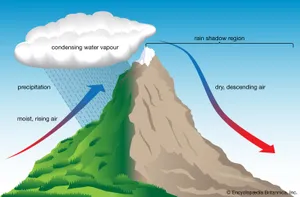
Orographic Lift: When the general circulation (like the Westerlies) hits a mountain range, air is forced upward. This creates heavy precipitation on the windward side and a “rain shadow” (dry zone) on the leeward side.

What is the relationship between the 500 HPA wind and pressure patterns?

Definitive Guide to Weather Map Analysis – Part 6 – The 500 mb Map – Convective Chronicles

In synoptic meteorology, the 500 hPa level (approximately 5,500 meters or 18,000 feet) is considered the “middle” of the atmosphere. At this height, the air is removed from the frictional drag of the Earth’s surface, allowing the relationship between wind and pressure to reach a near-perfect geostrophic balance.

1. Geostrophic Balance: Parallel Flow

Unlike surface winds that spiral across isobars due to friction, winds at the 500 hPa level flow parallel to the geopotential height contours.

This occurs because only two primary forces are in play:

Pressure Gradient Force (PGF): Acts perpendicular to the contours, pushing air from higher heights toward lower heights.
Coriolis Force (fV): Acts at a 90° angle to the right of the wind’s motion (in the Northern Hemisphere).

At 500 hPa, these two forces reach an equilibrium where they are equal in magnitude but opposite in direction. Consequently, if you stand with your back to the wind at this level, the area of lower pressure (lower heights) will be to your left.

2. Geopotential Height vs. Surface Pressure

At the surface, we look at pressure changes at a constant altitude. At 500 hPa, we look at altitude changes at a constant pressure.

Ridges (High Heights): Areas where the 500 hPa surface is physically higher in the atmosphere. These correspond to warmer, less dense columns of air.
Troughs (Low Heights): Areas where the 500 hPa surface “dips” lower toward the ground. These correspond to colder, denser columns of air.

The wind speed is determined by the spacing of the contours. Where the height gradient is steepest (contours are close together), the PGF is strongest, resulting in higher wind speeds—often indicating the presence of a jet streak.

3. Rossby Waves and Vorticity

The 500 hPa pattern is defined by long-wave undulations known as Rossby Waves. The relationship between the wind and these curves introduces the concept of vorticity (the “spin” of the air):

Trough Axes: As wind moves through a trough, it gains cyclonic (positive) vorticity. The area downwind (east) of a trough axis is characterized by Positive Vorticity Advection (PVA), which promotes rising air and surface cyclogenesis.
Ridge Axes: As wind moves over a ridge, it gains anticyclonic (negative) vorticity. The area downwind of a ridge axis experiences Negative Vorticity Advection (NVA), which promotes sinking air and surface high pressure.

4. The “Steering” Relationship

Because the 500 hPa level represents the bulk motion of the troposphere, it acts as the steering flow for surface weather systems.

Surface cyclones typically track along the path of the 500 hPa flow.
The speed of surface systems is generally about 50% of the 500 hPa wind speed.

Summary Table: 500 hPa vs. Surface

Feature	Surface (1000 hPa)	Upper Air (500 hPa)
Primary Forces	PGF, Coriolis, Friction	PGF, Coriolis
Wind Direction	Across isobars (10°–40°)	Parallel to contours
Map Features	Isobars (Pressure)	Geopotential Heights
Vertical Motion	Convergence/Divergence	Vorticity Advection

What is the “dishpan” experiment?

GS 109: Modeling Global Atmospheric Circulation – Columbia Gorge Community College

The “dishpan” experiment is a classic laboratory simulation used in geophysical fluid dynamics to model the general circulation of Earth’s atmosphere. Developed primarily by Dave Fultz at the University of Chicago in the late 1940s and 1950s, the experiment uses a rotating, heated vessel of fluid to demonstrate how planetary rotation and temperature gradients create the complex wind patterns we see on weather maps.

1. The Experimental Setup

The experiment consists of a circular, flat-bottomed pan (the “dishpan”) filled with water or another fluid. It simulates the Earth’s hemisphere using the following mechanics:

The Temperature Gradient: The outer rim of the pan is heated (representing the warm Equator), while the center is cooled (representing the cold Pole).
The Rotation: The entire pan is placed on a turntable and rotated at various speeds to simulate the Earth’s rotation and the resulting Coriolis effect.
Visualization: Aluminum powder or dyes are added to the water, and a camera rotating with the pan captures the flow patterns.

2. Key Findings: The Two Flow Regimes

The most significant outcome of the dishpan experiment was the discovery that atmospheric circulation transitions between two distinct states based on the rate of rotation and the intensity of the temperature gradient.

The Hadley Regime (Slower Rotation)

When the pan rotates slowly, the fluid follows a simple, symmetric path. It rises at the heated rim, flows toward the center at the surface, sinks at the cold center, and returns along the bottom. This is a laboratory confirmation of the single-cell model, where heat is transported directly by a steady meridional overturning.

The Rossby Regime (Faster Rotation)

As the rotation speed increases, the simple symmetric flow becomes unstable. The fluid begins to form undulating, wave-like patterns.

Meanders: The flow develops “kinks” that look remarkably like Rossby waves in the upper atmosphere.
Eddies: At high speeds, these waves break off into closed circles, simulating high and low-pressure systems (cyclones and anticyclones).
Jet Streams: Narrow bands of high-velocity flow form along the boundaries of these waves, mimicking the atmospheric jet streams.

3. Why It Matters to Meteorology

The dishpan experiment was revolutionary because it proved that the complex “wavy” nature of our weather isn’t caused by the shape of continents or the presence of oceans (since the pan has neither). Instead, it demonstrated that:

Fundamental Physics: Global weather patterns are a fundamental result of a fluid attempting to conserve angular momentum while being subjected to a temperature gradient on a rotating body.
The Rossby Number (Ro): The experiment helped define the dimensionless Rossby Number, which describes the ratio of inertial forces to Coriolis forces:

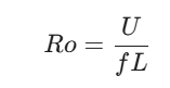
where U is velocity, f is the Coriolis parameter, and L is the length scale. This number tells meteorologists whether the flow will be straight (Hadley-like) or wavy (Rossby-like).

4. Modern Applications

Today, while we use massive supercomputers for Numerical Weather Prediction (NWP), physical “dishpan” simulations are still used in research to study:

Planetary Atmospheres: Modeling the banded winds of Jupiter or the polar vortex on Mars.
Oceanic Circulation: Understanding how deep-sea currents interact with the Earth’s rotation.
Climate Stability: Investigating how changing the temperature gradient (Global Warming) might shift the atmosphere from one flow regime to another.

What are the jet streams?

What Is the Jet Stream? – NOAA SciJinks

Jet streams are narrow bands of fast-moving air in the upper atmosphere that circle the globe from west to east. They act as the “rivers of air” that separate large masses of cold air from warm air, playing a critical role in steering weather systems and affecting aviation.

1. Physical Characteristics

A typical jet stream is thousands of kilometers long, a few hundred kilometers wide, and often less than five kilometers thick.

Altitude: They are usually found near the tropopause (the boundary between the troposphere and the stratosphere), typically between 9 km and 16 km (30,000 to 52,000 feet).
Speed: Winds within the jet stream must exceed 92 km/h (57 mph) to be formally classified as such, though they frequently reach speeds over 320 km/h (200 mph), especially during winter when temperature gradients are steepest.

2. Why Jet Streams Form

Jet streams are the result of two primary physical drivers: the horizontal temperature gradient and the rotation of the Earth.

The Temperature Gradient

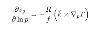
Jet streams form where large bodies of air with significantly different temperatures meet. The greater the temperature difference, the stronger the pressure gradient aloft. This relationship is defined by the Thermal Wind Equation, which shows that vertical wind shear is proportional to the horizontal temperature gradient:

The Coriolis Effect and Conservation of Momentum

As air moves poleward in the upper branches of the atmospheric cells, the Coriolis effect deflects it to the right (in the Northern Hemisphere). Because the air is moving closer to the Earth’s axis of rotation, it must speed up to conserve angular momentum, resulting in high-velocity westerly winds.

3. The Four Main Jet Streams

Earth typically has four primary jet streams, two in each hemisphere:

Polar Jet Stream: Located near 60° latitude. It forms at the Polar Front, where cold polar air meets warmer mid-latitude air. This jet is the most influential for weather in North America, Europe, and Asia.
Subtropical Jet Stream: Located near 30° latitude. It forms at the poleward limit of the Hadley Cell. It is generally higher in altitude and weaker than the polar jet, though it can merge with it during intense storm cycles.

4. Rossby Waves and Weather “Steering”

Jet streams do not flow in straight lines; they follow undulating paths called Rossby Waves.

Ridges: When the jet stream curves toward the pole, it creates a ridge of high pressure, usually bringing warm, dry weather.
Troughs: When the jet stream “dips” toward the equator, it creates a trough of low pressure, often bringing cold air and stormy conditions.
Jet Streaks: These are localized pockets of even faster air within the jet stream. The entry and exit regions of these streaks are primary sites for the development of surface cyclones (low-pressure systems).

5. Significance in Aviation

The jet stream is a major factor in flight planning:

Tailwinds: Flying eastbound “with” the jet stream can significantly reduce flight time and fuel consumption.
Headwinds: Flying westbound “against” the jet stream requires more fuel and takes longer.
Clear Air Turbulence (CAT): Because the jet stream has high wind shear (rapid changes in wind speed over short distances), it is a frequent source of turbulence that cannot be detected by traditional radar.

How do jet streams form?

What is the jet stream and how does it affect the weather? – Met Office – Learn About Weather

Jet streams form through the interaction of two fundamental physical drivers: intense horizontal temperature gradients and the Coriolis effect. They are essentially the atmospheric response to the Earth’s attempt to balance energy between the warm tropics and the cold poles.

1. The Temperature Gradient & Pressure

The process begins with the uneven heating of the Earth. Where large masses of cold, dense polar air meet warm, buoyant tropical air, a sharp temperature gradient is created.

Vertical Expansion: Warm air columns are physically “taller” (less dense) than cold air columns.
Pressure Slope: Because the warm air column is taller, the pressure at high altitudes (e.g., 250 hPa) is higher over the tropics than it is over the poles at that same altitude.
Pressure Gradient Force (PGF): This creates a powerful PGF aloft that pushes air directly from the warm tropics toward the cold poles.

2. The Coriolis Effect & Geostrophic Balance

If the Earth did not rotate, this air would flow directly north and south. However, because the Earth rotates:

Deflection: As the air moves poleward, the Coriolis effect deflects it to the right in the Northern Hemisphere and to the left in the Southern Hemisphere.
Geostrophic Flow: Eventually, the PGF pushing poleward and the Coriolis force pulling equatorward reach an equilibrium. The air stops moving across the gradient and instead flows parallel to the temperature boundary.
The Result: A high-speed “river” of air flowing from west to east.

3. Conservation of Angular Momentum

As air in the upper branch of the Hadley Cell moves away from the equator, it moves closer to the Earth’s axis of rotation.

Just like a figure skater pulling in their arms to spin faster, the air must increase its eastward velocity to conserve angular momentum (L = mvr).
By the time this air reaches the subtropics (~30° latitude), it is moving fast enough to form the Subtropical Jet Stream.

4. The Thermal Wind Relationship

In meteorology, this formation is described by the Thermal Wind Equation. This principle states that the vertical shear (the change in wind speed with height) is directly proportional to the horizontal temperature gradient.

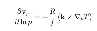
Where there is a steep temperature contrast (like the Polar Front), the wind speed must increase rapidly with height, reaching its maximum velocity just below the tropopause—this peak is the core of the jet stream.

5. Summary of Jet Stream Locations

The Earth typically maintains two primary jets per hemisphere due to these specific temperature boundaries:

Jet Stream	Latitude	Formation Mechanism
Polar Jet	~60°	The Polar Front (meeting of polar and mid-latitude air).
Subtropical Jet	~30°	Conservation of angular momentum at the edge of the Hadley Cell.

What are atmosphere-ocean interactions?

ESS 5. Lec. 11. The Atmosphere: Ocean Interactions – UCI Open

Atmosphere-ocean interactions refer to the continuous exchange of energy, momentum, and matter (such as water and CO2) across the interface between the air and the sea. Because the ocean covers over 70% of the Earth’s surface and has a much higher heat capacity than the atmosphere, it acts as the planet’s primary thermal reservoir and regulator.

1. Mechanisms of Exchange

The “conversation” between the two systems occurs through several physical processes:

Momentum Transfer (Wind Stress): As wind blows across the water, friction transfers kinetic energy to the surface. This creates waves and drives the large-scale oceanic gyres.
Heat Exchange:
- Sensible Heat: Direct transfer via conduction and convection due to temperature differences.
- Latent Heat: The most powerful transfer mechanism. Energy is absorbed by the ocean during evaporation and later released into the atmosphere during condensation (cloud formation), fueling storms.
Mass Exchange: This involves the water cycle (evaporation/precipitation) and the gas cycle, specifically the ocean’s role as a “carbon sink” for atmospheric CO₂.

2. Feedback Loops: Coupled Systems

The atmosphere and ocean are “coupled,” meaning a change in one system triggers a response in the other, often creating feedback loops.

The Walker Circulation

This is a longitudinal (east-west) circulation in the tropics. High pressure in the Eastern Pacific drives trade winds toward the Western Pacific. This pushes warm surface water westward, allowing cold, nutrient-rich water to well up in the east.

El Niño-Southern Oscillation (ENSO)

ENSO is the most famous example of atmosphere-ocean coupling.

El Niño: Trade winds weaken. The warm water “sloshes” back toward South America, shutting down upwelling. This alters the path of the jet stream, causing global weather shifts.
La Niña: Trade winds strengthen, pushing even more warm water west and intensifying the cold upwelling in the east.

3. The Thermohaline Circulation (The Global Conveyor Belt)

While wind drives surface currents, density differences (driven by temperature and salinity) drive deep-ocean circulation.

In the North Atlantic, cold, salty water sinks (downwelling).
The atmosphere influences this by cooling the water or adding fresh water (via melting ice), which can slow the “pump.”
In return, the ocean transports massive amounts of heat poleward (e.g., the Gulf Stream), keeping regions like Western Europe significantly warmer than their latitude would suggest.

4. Sea Surface Temperatures (SST) and Cyclogenesis

Ocean temperatures directly dictate atmospheric stability.

Tropical Cyclones: Hurricanes and typhoons require SSTs of at least 26.5°C to form. The ocean provides the “fuel” (latent heat), while the atmosphere provides the “engine” (vorticity and lift).
Marine Boundary Layer: Cold ocean currents (like the California Current) stabilize the air above them, leading to persistent coastal fog and suppressed rainfall.

5. Summary of Interactions

Interaction Type	Atmospheric Impact	Oceanic Impact
Wind Stress	Energy dissipation	Surface currents & upwelling
Evaporation	Latent heat for storms	Increased salinity (density)
Precipitation	Moisture removal	Decreased salinity
CO₂ Absorption	Greenhouse gas reduction	Ocean acidification

What is the relationship between the wind and surface ocean currents?

Oceans and climate – European Space Agency, ESA

The relationship between wind and surface ocean currents is primarily one of momentum transfer. When wind blows over the ocean, friction between the air and the water drags the surface layer along, initiating a complex chain of physical reactions governed by the Earth’s rotation.

While it might seem that water should move in the same direction as the wind, the reality is a bit more “twisted” due to the Coriolis effect.

1. The Ekman Spiral and Transport

The most fundamental principle connecting wind and water is the Ekman Spiral. When wind pushes the surface water, the Coriolis effect deflects that water to the right in the Northern Hemisphere (and to the left in the Southern Hemisphere).

Surface Layer: The very top layer of water moves at roughly a 45° angle to the wind direction.
The Spiral: As you go deeper, each subsequent layer of water is pushed by the layer above it. Because of friction and the Coriolis effect, each deeper layer moves even more slowly and is deflected even further to the right.
Ekman Transport: When you average the movement of the entire influenced water column (the Ekman layer), the net transport of water is 90° to the right of the wind direction in the Northern Hemisphere.

2. Geostrophic Gyres

On a global scale, the prevailing winds (Trade Winds and Westerlies) drive the large-scale circular patterns known as Gyres.

Wind Input: The Westerlies (at 40°–60°) push water eastward, while the Trade Winds (at 0°–30°) push water westward.
Convergence: Because of Ekman transport, water is pushed toward the center of the ocean basins from both the north and the south.
The “Hill” of Water: This creates a subtle “hill” or dome of water in the middle of the ocean (often about 1 meter high).
Geostrophic Balance: Gravity tries to pull the water down the hill, but the Coriolis effect deflects it. The result is a circular flow around the hill—a Geostrophic Current.

3. Coastal Upwelling and Downwelling

The 90° relationship between wind and water transport is most visible along coastlines, where it directly impacts marine ecosystems and local weather.

Upwelling: If the wind blows parallel to a coast such that Ekman transport moves water away from the shore, cold, nutrient-rich water from the deep must rise to replace it.
- Example: Winds blowing south along the California coast.
Downwelling: If the wind blows such that Ekman transport pushes water toward the shore, the water “piles up” and is forced downward. This results in nutrient-poor but oxygen-rich surface water being sent to deeper levels.

4. Western Boundary Currents

The interaction between wind and the Earth’s rotation also causes Western Boundary Intensification. Because the Coriolis effect increases with latitude, the gyres are “squeezed” against the western side of ocean basins.

This creates fast, narrow, and deep currents like the Gulf Stream or the Kuroshio Current. These currents act as the ocean’s equivalent of the atmospheric Jet Stream, transporting massive amounts of tropical heat toward the poles.

Summary of Wind-Current Relationships

Feature	Wind Driver	Water Response
Surface Direction	Wind Velocity	45° deflection from wind
Net Transport	Wind Stress	90° deflection (Ekman Transport)
Gyre Rotation	Trades & Westerlies	Clockwise (NH) / Counter-clockwise (SH)
Vertical Motion	Coastal Winds	Upwelling (Away from shore) / Downwelling (Toward shore)

What is upwelling?

Introduction to Upwelling – Ten Minute Team Tips with Bill Ferriter

Upwelling is an oceanographic phenomenon where deep, cold, and typically nutrient-rich water rises toward the surface to replace warmer surface water. This process is a direct result of the interaction between wind, the Earth’s rotation, and coastal geography.

While it covers less than 1% of the ocean’s surface, upwelling zones are biological powerhouses, supporting roughly 20% of the world’s fish catch.

1. The Physics: Ekman Transport

The primary driver of upwelling is Ekman Transport. As we discussed with surface currents, when wind blows across the ocean, the Coriolis effect deflects the net movement of the water column 90° to the right in the Northern Hemisphere (and 90° to the left in the Southern Hemisphere).

Coastal Upwelling

This occurs when winds blow parallel to a coastline in a specific direction:

Wind Direction: Along the west coast of a continent (like California or Peru), winds blowing toward the equator (southerly in the NH) push surface water.
Deflection: Ekman transport moves that surface water offshore (away from the land).
Replacement: To fill the “void” left by the departing surface water, denser, colder water from the depths (usually from 100–300 meters) is pulled upward.

2. Equatorial Upwelling

Upwelling also occurs in the open ocean, most notably along the equator.

The Trade Winds blow from the east toward the west in both hemispheres.
Due to the Coriolis effect, surface water is deflected northward in the Northern Hemisphere and southward in the Southern Hemisphere.
This “divergence” at the equator forces deep water to rise to the surface, creating a distinct “cold tongue” of water across the central Pacific.

3. Biological and Climate Impacts

Upwelling is critical because it acts as a “nutrient pump” for the ocean.

The Nutrient Pump: Deep water is rich in nitrates and phosphates (from the decomposition of organic matter that sank long ago). When this hits the “photic zone” (where sunlight penetrates), it triggers massive blooms of phytoplankton.
The Food Web: These blooms support vast populations of zooplankton, fish, and marine mammals.
Climate Regulation: Because upwelled water is significantly colder than the surrounding surface, it stabilizes the atmosphere above it. This often leads to:
- Coastal Fog: Common in places like San Francisco or the Skeleton Coast of Namibia.
- Aridity: The cold water inhibits the vertical convection needed for rain, contributing to the dryness of coastal deserts (like the Atacama).

4. Upwelling and ENSO

Upwelling is highly sensitive to changes in global wind patterns. During an El Niño event:

The Trade Winds weaken or reverse.
The “push” that drives Ekman transport stops.
Upwelling shuts down along the South American coast.
Result: Surface temperatures rise, and the nutrient supply is cut off, leading to a collapse of local fisheries and significant shifts in global weather patterns.

Summary of Upwelling Types

Type	Location	Forcing Mechanism	Result
Coastal	Continental Margins	Along-shore winds + Ekman Transport	Highly productive fisheries
Equatorial	0° Latitude	Divergence of North/South Trade Winds	“Cold tongue” in the Pacific
Large-scale	Southern Ocean	Strong Westerlies around Antarctica	Global nutrient redistribution

What are El Nino, La Nina, and the Southern Oscillation?

What is ENSO, El nino, La nina, Southern Oscillation, Walker Circulation | UPSC / IAS – Amit Sengupta

Together, these phenomena form ENSO (El Niño-Southern Oscillation), a single “coupled” ocean-atmosphere system in the tropical Pacific that serves as the Earth’s most powerful driver of year-to-year climate variability.

While the ocean changes (El Niño/La Niña) and the atmosphere changes (Southern Oscillation) are often discussed separately, they are effectively two sides of the same coin.

1. The “Normal” State: Walker Circulation

To understand the anomalies, we must first look at the neutral state of the Pacific.

The Atmosphere: Strong Trade Winds blow from east to west (South America toward Indonesia).
The Ocean: These winds push warm surface water westward, “piling it up” in the Western Pacific. This causes cold, nutrient-rich water to rise (upwelling) along the coast of South America.
The Result: A “Warm Pool” in the west (triggering heavy rain) and a “Cold Tongue” in the east (keeping it dry).

2. El Niño: The Warm Phase

El Niño (Spanish for “The Boy Child”) occurs when the tropical Pacific becomes unusually warm.

The Mechanism: The Trade Winds weaken or even reverse. The “pile” of warm water in the west sloshes back toward the east.
Atmospheric Shift: The rising air and heavy rainfall move from Indonesia toward the Central and Eastern Pacific.
Oceanic Impact: Upwelling off the coast of South America shuts down. This deprives the surface of nutrients, often leading to a collapse in local fisheries.
Global Weather: Typically brings wetter conditions to the southern US and South America, while causing droughts in Australia and Indonesia.

3. La Niña: The Cold Phase

La Niña (“The Girl Child”) is essentially an intensification of the “normal” state.

The Mechanism: The Trade Winds become exceptionally strong, pushing even more warm water into the Western Pacific.
Oceanic Impact: Upwelling in the Eastern Pacific intensifies, making the “Cold Tongue” even colder than usual.
Global Weather: Often leads to drought in the southern US, heavier monsoons in SE Asia, and cooler, stormier winters in the Northern US and Canada (including the Pacific Northwest).

4. The Southern Oscillation (The “S.O.” in ENSO)

While El Niño and La Niña describe ocean temperatures, the Southern Oscillation describes the atmospheric pressure flip-flop that accompanies them. It is measured by the SOI (Southern Oscillation Index), which compares air pressure between Tahiti (East) and Darwin, Australia (West).

Phase	Pressure in Tahiti	Pressure in Darwin	SOI Value
Normal / La Niña	High	Low	Positive (+)
El Niño	Low	High	Negative (-)

5. Summary of ENSO Relationship

Feature	Neutral	El Niño	La Niña
Trade Winds	Moderate	Weak / Reversed	Very Strong
Eastern Pacific SST	Cool	Warm	Very Cold
Thermocline	Slanted	Flattened	Steeply Slanted
Upwelling	Normal	Suppressed	Enhanced
Rainfall	Western Pacific	Central/Eastern Pacific	Western Pacific (Heavy)

Why It Matters

Because the Pacific is so vast, these shifts move the Jet Stream. For instance, during an El Niño, the Pacific Jet Stream often becomes more linear and shifts south, steering storms into California and the Southern US. During La Niña, the jet often becomes more “wavy,” allowing cold Arctic air to spill further south into the northern plains.

What is the Pacific Decadal Oscillation?

What on Earth is the Inter-decadal Pacific Oscillation? – Dr Gilbz

The Pacific Decadal Oscillation (PDO) is a long-term ocean-atmosphere climate pattern that describes shifts in sea surface temperatures (SST) in the North Pacific Ocean (north of 20°N). While it shares some visual similarities with ENSO (El Niño/La Niña), it operates on a much longer timescale—typically cycles of 20 to 30 years—and is centered in the mid-latitudes rather than the tropics.

Think of the PDO as a “background state” that can either amplify or dampen the effects of shorter-term weather patterns like El Niño.

1. The Two Phases of the PDO

The PDO is defined by the spatial arrangement of warm and cold water across the North Pacific basin.

The Positive (Warm) Phase

During a positive phase, the SST pattern looks like a “horseshoe” of warmth along the west coast of North America.

The “Horseshoe”: Warm water hugs the coast of Alaska, British Columbia, and the Western United States.
The Center: A pool of unusually cold water forms in the central and western North Pacific.
Atmospheric Impact: This phase is often associated with a deeper-than-normal Aleutian Low, which steers more storms toward the coast of Alaska and can lead to warmer, drier winters in the Pacific Northwest and Western Canada.

The Negative (Cool) Phase

During a negative phase, the pattern reverses.

The “Horseshoe”: Cold water replaces the warmth along the North American coast.
The Center: The central North Pacific becomes warmer than average.
Atmospheric Impact: This typically correlates with a weaker Aleutian Low and can lead to cooler, wetter conditions in the Pacific Northwest.

2. PDO vs. ENSO: Scale and Duration

While the SST maps for a Positive PDO and an El Niño look remarkably similar, they are distinct phenomena:

Feature	ENSO (El Niño/La Niña)	PDO
Primary Location	Tropical Pacific	North Pacific (Extra-tropics)
Timescale	2 to 7 years	20 to 30 years
Main Driver	Trade Wind / Upwelling shifts	Mid-latitude jet stream / Aleutian Low
Predictability	High (6–12 months)	Low (decadal variability)

3. The “Amplifier” Effect

The PDO is most significant for its ability to modify the impacts of El Niño and La Niña.

Constructive Interference: When the PDO and ENSO are in the same phase (e.g., Positive PDO + El Niño), the weather impacts—such as droughts or heavy rainfall—tend to be more extreme and persistent.
Destructive Interference: When they are in opposite phases (e.g., Positive PDO + La Niña), they can “cancel each other out,” leading to more moderate or unpredictable weather seasons.

4. Ecological and Economic Impact

The PDO has massive implications for marine biology and the economy, particularly in the North Pacific.

Fisheries: Historically, the Positive Phase favors Alaskan Salmon populations, while the Negative Phase favors West Coast Salmon (Washington/Oregon/BC).
Agriculture: Long-term “warm” phases can lead to multi-decadal “megadroughts” in the Southwestern United States by influencing the persistent position of the jet stream.

5. Current Scientific Debate

There is ongoing research into whether the PDO is a single physical mechanism or simply the cumulative “echo” of several other processes, including:

ENSO Teleconnections: Tropical El Niño events sending “waves” of energy into the North Pacific.
Atmospheric Bridge: Changes in the Aleutian Low changing the mixing of the ocean surface.
The “Stochastic” View: The PDO may just be the sum of random, short-term weather fluctuations that appear to have a long-term signal.

What are the North Atlantic and Arctic Oscillations?

Arctic Oscillation North Atlantic Oscillation com – Idiocracy

The North Atlantic Oscillation (NAO) and the Arctic Oscillation (AO) are closely related atmospheric pressure patterns that dictate the strength of the “wall” of air—the jet stream—that keeps cold Arctic air contained at the poles.

While the AO describes the pressure state of the entire Northern Hemisphere, the NAO focuses specifically on the North Atlantic sector.

1. The Arctic Oscillation (AO)

The AO is a measure of the pressure difference between the Arctic and the mid-latitudes. It acts like a “gatekeeper” for cold air.

Positive Phase (+AO): A deep low-pressure system sits over the North Pole, while high pressure sits over the mid-latitudes. This creates a strong, stable jet stream that acts as a tight ring, trapping frigid air in the Arctic.
- Result: Milder winters for North America and Europe.
Negative Phase (-AO): The pressure difference weakens. The polar low “fills” (pressure rises), and the jet stream becomes wavy and sluggish.
- Result: The “gate” opens, allowing the Polar Vortex to spill southward, leading to record-breaking cold snaps and snowstorms in mid-latitude regions.

2. The North Atlantic Oscillation (NAO)

The NAO is a more localized version of the AO, defined by the pressure gradient between the Icelandic Low and the Azores High.

Positive Phase (+NAO): Both the Icelandic Low and the Azores High are stronger than usual. This “pumps” a strong jet stream across the Atlantic toward Northern Europe.
- Result: Eastern North America sees warmer, wetter conditions, while Northern Europe stays mild and stormy.
Negative Phase (-NAO): Both pressure systems weaken. The jet stream slows down and “buckles.”
- Result: This often leads to high-pressure blocking over Greenland (the “Greenland Block”). This forces cold air to plunge into the Eastern U.S. and Southern Europe, frequently resulting in “Nor’easters” and heavy snow.

3. Current Status (March 2026)

As of early March 2026, the atmosphere is in a highly dynamic state:

Positive Trends: Recent observations show both the AO and NAO are currently in a positive phase (AO at +1.24 and NAO at +1.50). This explains the current “zonal” flow—a flatter, faster jet stream—that is bringing milder Pacific air across much of the central and southern United States.
The “Polar Vortex” Threat: Despite the positive surface indices, a Sudden Stratospheric Warming (SSW) event occurred in late February 2026. This has significantly destabilized the Polar Vortex aloft.
Forecast: While the indices are positive now, models are tracking a potential shift toward a negative AO/NAO later in March as the stratospheric disruption “filters down” to the surface. This could lead to a final “wintry punch” for Eastern Canada and the Northern U.S. after a period of early spring warmth.

4. Key Differences

Feature	Arctic Oscillation (AO)	North Atlantic Oscillation (NAO)
Geographic Scope	Entire Northern Hemisphere (20°N–90°N)	North Atlantic (Subtropical to Subpolar)
Pressure Centers	Polar Low vs. Mid-latitude High	Icelandic Low vs. Azores High
Primary Impact	Global Polar Vortex containment	Steering of Atlantic storm tracks
Current Phase	Positive (as of March 4, 2026)	Positive (as of March 4, 2026)

How is anthropogenic climate change affecting the atmospheric general circulation?

Canada’s Most Destructive Wildfire! | Inside the Battle Against ‘The Beast’ | FULL DOCUMENTARY –
Curious? Science and Engineering

The impact of anthropogenic climate change on the atmospheric general circulation is often described as a “tug-of-war” between different physical drivers. While the core mechanics—the Hadley, Ferrel, and Polar cells—remain intact, their boundaries, intensity, and stability are shifting as the planet warms.

1. Expansion of the Hadley Cell

One of the most robustly observed changes is the poleward expansion of the tropical Hadley cells.

The Mechanism: As the troposphere warms and the tropopause rises, the point at which air becomes unstable and sinks (the subtropical high-pressure belt) moves toward the poles.
The Result: The world’s dry subtropical zones are shifting into higher latitudes. This has significant implications for Mediterranean-style climates, contributing to increased aridity in regions like the Southwestern United States, Southern Africa, and parts of Australia.

2. Arctic Amplification and the Jet Stream

The Arctic is warming nearly four times faster than the global average—a phenomenon known as Arctic Amplification. This reduces the temperature gradient between the equator and the North Pole.

Weakening the “Engine”: Since the strength of the jet stream is driven by this temperature contrast (via the Thermal Wind relationship), a smaller gradient results in a weaker, more “sluggish” jet stream.
Rossby Wave Amplification: A weaker jet stream is more prone to developing large, slow-moving meanders (Rossby waves). These “lazy” waves can lead to Atmospheric Blocking, where weather patterns (like heatwaves or stalled low-pressure systems) get stuck over a region for weeks at a time.

3. The “Tug-of-War” on the Mid-Latitude Jets

While Arctic warming tries to push the jet stream equatorward or make it wavier, warming in the upper tropical troposphere acts in the opposite direction.

Tropical Warming: The upper levels of the tropics are warming faster than the surface, which actually increases the temperature gradient in the upper atmosphere.
Poleward Shift: In many climate models, the net result for the Southern Hemisphere and the North Atlantic is a poleward shift of the mid-latitude storm tracks. This moves life-sustaining rain away from mid-latitude regions toward the sub-polar regions.

4. Intensification of the Hydrological Cycle

A warmer atmosphere can hold more water vapor (governed by the Clausius-Clapeyron relationship, approximately 7% more moisture per 1°C of warming).

The “Rich Get Richer” Effect: General circulation models show that areas of moisture convergence (like the ITCZ) are seeing more intense rainfall, while areas of divergence (the Subtropical Highs) are experiencing enhanced evaporation and drought.
Latent Heat Feedback: As more water vapor condenses in the tropics, it releases more latent heat, which can further energize the Hadley cell circulation, potentially offsetting some of the weakening caused by Arctic warming.

5. Summary of Circulation Shifts

Circulation Feature	Observed/Projected Change	Primary Impact
Hadley Cell	Poleward expansion	Expansion of deserts/subtropical aridity.
ITCZ	Narrowing and intensification	More extreme tropical rainfall events.
Jet Stream	Increased “waviness” (meandering)	Persistent weather extremes (heatwaves/floods).
Storm Tracks	Poleward migration	Changes in winter precipitation for mid-latitudes.
Walker Circulation	Potential weakening	Altered frequency/intensity of El Niño events.

6. The 2026 Context

Current observations in 2026 continue to monitor the Atlantic Meridional Overturning Circulation (AMOC). There is increasing concern that the slowing of this “oceanic conveyor belt” (due to freshwater influx from Greenland) is starting to decouple from the atmospheric general circulation, potentially leading to more erratic “flash” transitions in North Atlantic weather patterns.

Solved Problems

Atmospheric Dynamics & Synoptic Meteorology

1. The Geostrophic Balance Calculation

Problem: At a latitude of 45°N, the pressure gradient is measured at 3 hPa per 100 km. If the air density (ρ) is 1.2 kg/m³, calculate the geostrophic wind speed (V_g).
Solution: Use V_g = (1 / (fρ)) * (ΔP / Δn). With f ≈ 10^-4 s^-1 and ΔP/Δn = 0.003 Pa/m, V_g ≈ 25 m/s (≈ 90 km/h).

2. Thermal Wind and Jet Stream Intensity

Problem: A strong temperature gradient exists between 40°N and 50°N. If the mean temperature of the layer decreases by 10°C over 1,000 km, how does the westerly wind component change between 850 hPa and 250 hPa?
Solution: Applying the Thermal Wind Equation, a stronger horizontal temperature gradient (∂T/∂y) leads to a significant increase in geostrophic wind with height (∂u_g/∂z), typically resulting in the formation of a jet streak at the tropopause.

3. Vorticity and Cyclogenesis

Problem: An upper-level trough is moving over the Rockies into the Alberta plains. Explain why the area immediately east of the trough axis is favorable for surface low-pressure development.
Solution: This area experiences Positive Vorticity Advection (PVA). According to the Omega Equation, PVA promotes large-scale ascending motion, which lowers surface pressure and initiates cyclogenesis.

4. The Chinook Arch and Adiabatic Warming

Problem: Air at 0°C and 100% humidity at sea level rises over a 3,000m mountain range and descends into Calgary (approx. 1,000m elevation). Calculate the final temperature.
Solution: Air cools at the Saturated Adiabatic Lapse Rate (~6°C/km) during ascent and warms at the Dry Adiabatic Lapse Rate (10°C/km) during descent. The latent heat released during condensation results in a much warmer, drier wind on the leeward side (the Föhn effect).

5. Rossby Wave Speed

Problem: Calculate the phase speed (c) of a planetary Rossby wave with a wavelength of 5,000 km at 45°N, where the westerly flow (u) is 30 m/s.
Solution: Use the Rossby wave formula: c = u – β L² / 4π². If the westward “retrogression” term exceeds the eastward flow, the wave will move west; otherwise, it moves east at a slower speed than the background wind.

Geomatics & Physical Remote Sensing

6. Convergence of Meridians in Surveying

Problem: When performing a long-baseline survey in Alberta, why must “convergence of meridians” be accounted for when calculating azimuths?
Solution: Because meridians converge toward the poles, a straight line (great circle) does not maintain a constant bearing. The correction is Δα = Δλsinϕ_mid.

7. GNSS Ionospheric Delay

Problem: How does a dual-frequency GNSS receiver eliminate ionospheric error compared to a single-frequency unit?
Solution: The ionosphere is a dispersive medium; the delay is proportional to 1/f². By comparing the phase/code delay of L1 and L2 frequencies, the receiver can solve for the Total Electron Content (TEC) and remove the delay.

8. Orthorectification and Terrain Displacement

Problem: An aerial photo is taken over the Canadian Rockies. A mountain peak 1,000m above the datum appears shifted outward from the center. How is this corrected?
Solution: Through Orthorectification, using a Digital Elevation Model (DEM) to mathematically shift pixels from their perspective position to their true planimetric (X, Y) position, removing relief displacement.

9. LiDAR Pulse Penetration

Problem: In a forestry application, how do you distinguish between the “Canopy Top” and the “Ground Truth” using a single LiDAR pulse?
Solution: Analyze the multi-return signal. The first return typically represents the highest canopy, while the last return (if the pulse isn’t fully attenuated) represents the forest floor.

10. Map Projection Distortion (UTM Zone 12)

Problem: Why is the scale factor ($k$) exactly 0.9996 at the Central Meridian of a UTM zone?
Solution: To minimize overall distortion across the 6° zone. By making the central meridian slightly “smaller,” the projection achieves two lines of zero distortion (secant lines) rather than just one, balancing scale error across the zone.

IT Systems & Environmental Monitoring

11. High-Availability Weather Data Clusters

Problem: You are designing a server architecture for “Cavanu Starline” to handle 10,000 concurrent API requests for GFS data. How do you prevent a single point of failure?
Solution: Implement a Load Balancer (e.g., Nginx or HAProxy) in front of a cluster of redundant web servers with a distributed database (like Redis for caching) to ensure high availability and low latency.

12. IoT Sensor Calibration Drift

Problem: A network of 50 remote weather sensors shows a consistent 2°C warm bias over six months. What IT protocol can automate the correction?
Solution: Implement an Edge Computing script that compares local readings against a “Golden Standard” (e.g., an ECCC station) and applies a dynamic offset (bias correction) via a centralized configuration management tool.

13. Bandwidth Optimization for Satellite Imagery

Problem: You need to serve high-resolution GOES-16 satellite imagery on your website without slowing down mobile users.
Solution: Use Cloud-Optimized GeoTIFFs (COG) or a Tile Map Service (TMS). This allows the browser to request only the specific “tiles” and resolution levels needed for the user’s current zoom extent.

14. Automated Scripting for Data Ingestion

Problem: Write a logic flow to ingest GRIB2 weather files from an FTP server every 6 hours, ensuring partially downloaded files aren’t processed.
Solution: Use a Python script with ftplib that downloads to a .tmp extension, verifies the file size/checksum, and only renames it to .grib2 upon successful completion (atomic operation).

import os
import hashlib
from ftplib import FTP

def download_grib2(host, remote_path, local_filename):
temp_filename = f”{local_filename}.tmp”
final_filename = f”{local_filename}.grib2″

try:
    with FTP(host) as ftp:
        ftp.login()  # Add credentials if not anonymous

        # 1. Get remote file size for verification
        remote_size = ftp.size(remote_path)

        # 2. Perform the download
        print(f"Downloading {remote_path}...")
        with open(temp_filename, 'wb') as f:
            ftp.retrbinary(f"RETR {remote_path}", f.write)

        # 3. Verify File Size
        local_size = os.path.getsize(temp_filename)
        if remote_size != local_size:
            raise IOError(f"Size mismatch: {remote_size} (remote) vs {local_size} (local)")

        # 4. Atomic Rename
        # os.replace is atomic on most platforms, preventing partial file reads
        os.replace(temp_filename, final_filename)
        print(f"Success! File saved as {final_filename}")

except Exception as e:
    print(f"Error: {e}")
    if os.path.exists(temp_filename):
        os.remove(temp_filename)

15. RISC-V vs. x86 in Remote Weather Stations

Problem: Why might a RISC-V architecture be preferable for a solar-powered weather station in the high Arctic?
Solution: RISC-V allows for a highly optimized, low-power instruction set tailored specifically for sensor polling, reducing the “computational tax” of unnecessary legacy x86 instructions and extending battery life.

Advanced Synthesis (Type 1 Civilization & Energy)

16. Ocean Thermal Energy Conversion (OTEC) Efficiency

Problem: Calculate the theoretical maximum efficiency (η) of an OTEC plant where the surface water is 27°C and the deep water is 4°C.
Solution: Using the Carnot efficiency: η = 1 – (T_cold/T_hot) = 1 – (277K/300K) ≈ 7.6%. While low, the “fuel” (ocean heat) is nearly infinite.

17. Predicting Solar Flare Impact on Power Grids

Problem: A G5-class solar storm is detected. How does this impact high-voltage transmission lines in Calgary?
Solution: The storm induces Geomagnetically Induced Currents (GIC). Because the Earth’s magnetic field lines are nearly vertical at high latitudes, these currents can saturate transformer cores, leading to overheating and potential grid failure.

18. Polar Vortex Destabilization and Energy Demand

Problem: A Sudden Stratospheric Warming (SSW) is detected in February. How should a utility provider in Alberta prepare?
Solution: Expect a 2-week lag followed by a potential -30°C cold snap as the Polar Vortex dips south. Increase natural gas storage reserves and prepare for peak “heating degree day” (HDD) loads.

Meteorology Today Second Canadian Edition

Earth and Atmospheric Sciences