
What is differentiation in a single variable?
Earth and Atmospheric Sciences
Think of a derivative as the mathematical version of a “speedometer.” While algebra helps you find the average rate of change over a big chunk of time, calculus allows you to zoom in so far that you can see exactly how fast something is changing at a single, precise moment.
The Core Concept: Instantaneous Change

In simplest terms, a derivative measures the slope of a function at any given point.
- On a straight line: The slope is constant. If you’re walking at 3 mph, your “derivative” is always 3.
- On a curve: The slope is constantly changing. The derivative tells you the steepness of the curve at any specific x value.
How It Works (The Tangent Line)
To find the derivative at a point, we use a tangent line—a straight line that just barely touches the curve at that one spot.

- The Secant Line: In basic math, you pick two points and find the slope between them (rise / run).
- The Limit: In calculus, you move those two points closer and closer together until the distance between them is essentially zero.
- The Derivative: The result is the slope of the tangent line at that exact moment.
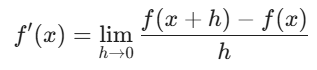
The Formal Definition
Mathematically, we represent this “closing the gap” using a limit. If f(x) is our function, the derivative f'(x) is defined as:
Real-World Examples
Derivatives are everywhere because everything in the universe is in motion or changing:
- Physics: If you have a formula for a car’s position, the derivative of that formula gives you its velocity. The derivative of velocity gives you acceleration.
- Economics: “Marginal cost” is just the derivative of the total cost function—it tells you how much it costs to produce just one more unit.
- Biology: Measuring the rate at which a population of bacteria grows over time.
Common Notations
You’ll see derivatives written in a few different ways depending on the textbook:
- Lagrange’s notation: f'(x) (read as “f prime of x”)
- Leibniz’s notation: dy / dx (read as “the derivative of y with respect to x”)
Fun Fact: Calculus was independently co-invented by Isaac Newton and Gottfried Wilhelm Leibniz in the 17th century. They spent years arguing over who got there first, but today we use a mix of both their systems!
What were the early methods of finding derivatives?
Before the formal “limit” definition was polished in the 19th century, mathematicians used some pretty clever (and sometimes controversial) workarounds. They knew they needed the slope of a curve at a single point, but they were stuck with the old algebraic rule that required two points.
Here is how the pioneers solved it:
1. Fermat’s “Adequality” (Pre-Calculus)
Before Newton or Leibniz were even born, Pierre de Fermat used a method called adequality. To find the peak of a curve, he would:
- Add a tiny amount (e) to his variable x.
- Set the original equation and the “nudged” equation almost equal to each other.
- Divide by e and then—this was the “magic” part—simply treat any remaining e as if it were zero.
2. Newton’s “Fluxions” and “Fluents”
Isaac Newton thought about calculus through the lens of physics and motion.
- Fluents: The variables (like x and y) that “flowed” over time.
- Fluxions: The speeds at which they flowed (their derivatives).
Newton used a tiny increment of time called “o”. He would calculate the change over time “o,” and at the end of the calculation, he would let “o” vanish.
3. Leibniz’s “Infinitesimals”
Gottfried Wilhelm Leibniz approached it geometrically. He imagined that a curve was actually made up of an infinite number of infinitely short straight line segments.
- He called the tiny change in vertical height dy.
- He called the tiny change in horizontal distance dx.
- The derivative was simply the ratio dy / dx.
The “Ghosts of Departed Quantities”
These early methods worked perfectly, but they had a major logical flaw: How can a number be small enough to ignore, but not be zero?
If you divide by dx (or Newton’s o), it can’t be zero, because you can’t divide by zero. But if you want it to disappear at the end, it has to be zero. This logical contradiction led Bishop George Berkeley to famously mock these tiny numbers as:
“…the ghosts of departed quantities.”
Comparison of Early Methods
| Method | Key Proponent | Concept Used |
| Adequality | Pierre de Fermat | Comparing “nearly equal” values. |
| Fluxions | Isaac Newton | Rates of flowing quantities over time. |
| Infinitesimals | Gottfried Leibniz | Ratios of infinitely small differences. |
It wasn’t until the 1800s that mathematicians like Augustin-Louis Cauchy developed the Limit, which finally explained how these “ghosts” worked without breaking the rules of math.
How can the derivative be considered a function?
This is the “aha!” moment in calculus. Up until now, we’ve talked about the derivative as the slope at one specific point. But if you calculate that slope for every possible point on a curve, those slopes form a pattern.
That pattern is, itself, a new function.
From Points to Patterns
Imagine you are driving a car on a hilly road.
- The original function f(x): This is the map of the road. It tells you your altitude at any horizontal distance x.
- The derivative function f'(x): This is your inclinometer. At any distance x, it tells you the exact steepness of the road.
If the road goes up, then down, then up again, your inclinometer will show a positive number, then zero at the peak, then a negative number. If you graph those inclinometer readings, you get the derivative function.
A Concrete Example: f(x) = x2
Let’s look at the classic parabola. The slope changes depending on where you are:
| If x is… | The Slope (Derivative) is… |
| -2 | -4 (Steeply downhill) |
| -1 | -2 (Gently downhill) |
| 0 | 0 (Flat bottom of the bowl) |
| 1 | 2 (Gently uphill) |
| 2 | 4 (Steeply uphill) |
Notice the pattern in the right column? Every slope is exactly double the x value. Instead of calculating the slope manually every time, we can just say:
f'(x) = 2x
Now, 2x is a function! You can plug any x into it, and it instantly spits out the slope of the original parabola at that spot.
Why Thinking of it as a Function Matters
When we treat the derivative as a function, we can perform calculus on the calculus.
- First Derivative (f’): Tells you the rate of change (Velocity).
- Second Derivative (f”): Tells you the rate of change of the rate of change (Acceleration).
- Third Derivative (f”’): Tells you how the acceleration is changing (in physics, this is literally called “Jerk”).
Summary: The Two Perspectives
- The “Value” Perspective: f'(3) is a single number representing the slope at x=3.
- The “Function” Perspective: f'(x) is a rule or “machine” that describes the slope for the entire domain of the original graph.
What are the differentiation formulas?
Instead of using the long “limit” definition every time, mathematicians developed differentiation rules. These are shortcuts that allow you to find the derivative function f'(x) almost instantly just by looking at the structure of the equation.
Here are the fundamental formulas you’ll use in a first-year calculus course.
1. The Basic Building Blocks
These rules cover the simplest types of functions, like constants and straight lines.
- The Constant Rule: The derivative of any constant number is always 0.
- Logic: A constant (like y = 5) is a flat horizontal line; its slope never changes.
- Formula: d (c) / dx = 0
- The Power Rule: This is the “workhorse” of calculus. To find the derivative of x raised to a power, bring the exponent down to the front and subtract one from the original exponent.
- Formula: d (xn) / dx = nxn-1
- Example: If f(x) = x3, then f'(x) = 3x2.
2. Rules for Combining Functions
When functions are added, multiplied, or divided, we use these “structural” rules.
| Rule | Formula | When to use it |
| Sum/Difference | d [f(x) ± g(x)] / dx = f'(x) ± g'(x) | When terms are added/subtracted. |
| Product Rule | d [f(x)g(x)] / dx = f'(x)g(x) + f(x)g'(x) | When two x-terms are multiplied. |
| Quotient Rule | d [f(x) / g(x)] / dx = (f'(x)g(x) – f(x)g'(x)) / [g(x)]2 | When one x-term is divided by another. |
3. Transcendental Functions (Trig & Logs)
Some functions don’t follow the Power Rule and have their own specific “identities.”
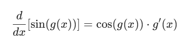
- Trigonometric Derivatives:
- d (sin x) / dx = cos x
- d (cos x) / dx = -sin x
- d (tan x) / dx = sec2x
- Exponential and Logarithmic:
- The Natural Exponential: d (ex) / dx = ex (This is the only function that is its own derivative!)
- The Natural Log: d (ln x) / dx = 1 / x
4. The “Boss Level”: The Chain Rule
This is used when you have a function inside another function, like sin(x2). You take the derivative of the “outside” function first, then multiply it by the derivative of the “inside” function.
A Quick Cheat Sheet
If you had to memorize just one, make it the Power Rule. It covers about 80% of introductory problems.
Pro Tip: When using the Quotient Rule, many students use the mnemonic: “Low D-High minus High D-Low, over the square of what’s below.” > (Low * d / dx High – High * d / dx Low)
What are rates of change in the natural and social sciences?
In the natural and social sciences, a rate of change is simply a mathematical description of how one variable responds to another. While we often think of change over time, rates can also describe how things change over distance, price, or concentration.
Calculus allows scientists to move from “average” rates (the total change) to “instantaneous” rates (what is happening right this second).
1. Physical Sciences (Physics & Chemistry)
In the physical world, rates of change describe the fundamental laws of motion and matter.
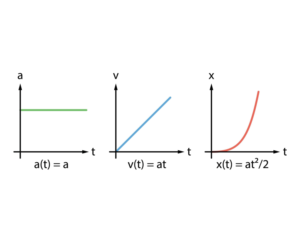
- Kinematics: As we touched on earlier, velocity is the rate of change of position, and acceleration is the rate of change of velocity.
- Thermodynamics: The rate of heat transfer (dQ / dt) tells engineers how quickly a cooling system must work to prevent an engine from melting.
- Chemistry (Reaction Kinetics): Chemists use derivatives to find the reaction rate—how fast reactants are consumed or products are created.
2. Biological Sciences
Biology is rarely static; it is defined by growth and decay.
- Population Dynamics: The Malthusian Growth Model uses derivatives to predict how a population (like bacteria or deer) will grow based on its current size.
- Equation snippet: dP / dt = rP (The change in population over time equals the growth rate times the current population).
- Pharmacokinetics: Doctors use rates of change to determine the half-life of a drug—how fast the concentration of medicine in your bloodstream drops over time.
- Epidemiology: During a pandemic, the “rate of infection” determines whether a healthcare system will be overwhelmed.
3. Social Sciences (Economics & Sociology)
In social sciences, rates of change help us understand human behavior and systems.
- Marginalism in Economics: This is the most famous use of derivatives in the social sciences.
- Marginal Cost: The cost of producing one more item.
- Marginal Utility: The satisfaction gained from consuming one more unit of a good.
- Psychology: The Weber-Fechner Law describes the rate at which our perception of a stimulus (like sound or light) changes relative to the actual intensity of the stimulus.
- Demographics: Sociologists look at the fertility rate or migration rate to predict how the “shape” of a society (its age distribution) will change in the coming decades.
Why “Instantaneous” Matters
In all these fields, knowing the average isn’t enough.
Example: If a dam is leaking, knowing that it leaked 1,000 gallons over 24 hours (the average) is less important than knowing if the rate of the leak is currently accelerating. If the derivative is increasing, the dam is about to fail.
Summary Table: Rates Across Disciplines
| Field | Dependent Variable (y) | Independent Variable (x) | The Derivative (dy/dx) |
| Physics | Position | Time | Velocity |
| Chemistry | Concentration | Time | Reaction Rate |
| Economics | Total Cost | Quantity | Marginal Cost |
| Biology | Population | Time | Growth Rate |
What are derivatives of trigonometric functions?
The derivatives of trigonometric functions describe how the ratios of a right triangle (or the coordinates on a unit circle) change as the angle θ changes. Because trig functions are periodic (they repeat in waves), their derivatives are also periodic functions.
1. The Core Six
In a standard calculus course, you will primarily work with these six formulas. Notice the patterns: every “Co-” function (Cosine, Cotangent, Cosecant) has a negative derivative.
| Function f(x) | Derivative f′(x) |
| sin(x) | cos(x) |
| cos(x) | -sin(x) |
| tan(x) | sec2(x) |
| cot(x) | -csc2(x) |
| sec(x) | sec(x) tan(x) |
| csc(x) | – csc(x) cot(x) |
2. Visualizing sin(x) and cos(x)
The relationship between Sine and Cosine is one of the most beautiful “loops” in math.
- At the peak of a Sine wave, the graph is flat (slope = 0). If you look at a Cosine graph at that same x value, it is crossing the x-axis (value = 0).
- Where the Sine wave is steepest (crossing the axis), the Cosine wave is at its maximum.
3. Geometric Interpretation (Unit Circle)
If you imagine a point moving around a unit circle at a constant speed, the derivative represents the velocity vector of that point.
- The y-coordinate is sin(θ).
- As you move, the vertical “velocity” of that point is exactly cos(θ).
- This is why trig derivatives are essential in physics for describing Simple Harmonic Motion (like a swinging pendulum or a vibrating guitar string).
4. Applying the Chain Rule
In the real world, you rarely see a simple sin(x). Usually, the angle is also a function, such as sin(3x2). In these cases, you must use the Chain Rule:
Example:
To find the derivative of y = tan(5x):
- The derivative of the “outside” (tan) is sec2.
- The derivative of the “inside” (5x) is 5.
- Result: y’ = 5sec2(5x).
5. Higher-Order Derivatives (The Loop)
Trig derivatives are unique because they cycle. If you keep taking the derivative of sin(x), you eventually get back to where you started:
- f(x) = sin(x)
- f'(x) = cos(x)
- f”(x) = -sin(x)
- f”'(x) = -cos(x)
- f(4)(x) = sin(x) (Back to the start!)
What is the chain rule?
The Chain Rule is the formula used to find the derivative of a composite function—essentially, a function wrapped inside another function.
If you think of a derivative as a “rate of change,” the Chain Rule is how you calculate the total change when one variable depends on a second, which in turn depends on a third.
1. The Core Concept: “Functions Inside Functions”
In algebra, a composite function looks like f(g(x)).
- The “Inner” Function: g(x)
- The “Outer” Function: f(u)
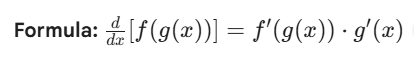
The Rule: To find the derivative, you take the derivative of the outside (leaving the inside alone), then multiply it by the derivative of the inside.
The Formal Formula
dy / dx = f'(g(x)) * g'(x)
2. A Real-World Analogy: The Gear System
Imagine three gears connected in a line: Gear A, Gear B, and Gear C.
- If Gear A turns 3 times as fast as Gear B…
- And Gear B turns 2 times as fast as Gear C…
- Then Gear A must turn 3 * 2 = 6 times as fast as Gear C.
The Chain Rule is simply that multiplication (3 * 2). You multiply the rates of change together to get the “total” rate of change.
3. How to Use It (Step-by-Step)
Let’s find the derivative of y = (3x2 + 1)4.
- Identify the layers:
- Outside: (something)4
- Inside: 3x2 + 1
- Differentiate the outside: Treat the inside like a single block. Using the Power Rule, the 4 comes down:
- 4(3x2 + 1)3
- Differentiate the inside: The derivative of 3x2 + 1 is 6x.
- Multiply them together:
- y’ = 4(3x2 + 1)3 * 6x
- Simplify:
- y’ = 24x(3x2 + 1)3
4. Leibniz’s Notation (The “Cancellation” Trick)
One reason Leibniz’s notation (dy / dx) is so popular is that it makes the Chain Rule look like simple fraction multiplication. If y depends on u, and u depends on x, then:
dy / dx = dy / du * du / dx
Mathematically, it looks as if the du terms “cancel out,” leaving you with dy / dx. While they aren’t actually fractions, this visual shorthand is incredibly helpful for keeping track of complex problems.
5. When do you need it?
You need the Chain Rule whenever a function is “modified” by something other than a plain x.
- Power Rule + Chain: (5x + 2)3
- Trig + Chain: cos(x2)
- Log + Chain: ln(7x – 3)
What is implicit differentiation?
Gemini said
Implicit differentiation is a technique used when you can’t (or don’t want to) isolate y on one side of an equation.
Most functions we’ve looked at so far are explicit, like y=x2+5. Here, y is isolated, and finding the derivative is straightforward. However, many mathematical relationships are implicit, meaning x and y are tangled together, like in the equation of a circle:
x2+y2=25
1. The Core Idea: y is a Function of x
The secret to implicit differentiation is treating y as an “invisible” function of x. Even if we don’t know exactly what y equals, we know it depends on x.
Because of this, every time you take the derivative of a term containing y, you must apply the Chain Rule. This means you differentiate the y term normally, then “tack on” a dxdy (or y′) at the end.
2. Step-by-Step Process
Let’s find the slope (dxdy) of the circle x2+y2=25:
- Differentiate both sides with respect to x.
- The derivative of x2 is 2x.
- The derivative of y2 is 2y⋅dxdy (Remember the Chain Rule!).
- The derivative of 25 is 0.
- Equation: 2x+2ydxdy=0
- Isolate the dxdy term.
- Subtract 2x from both sides: 2ydxdy=−2x
- Divide by 2y: dx / dy=2y−2x
- Simplify.
- dxdy=−yx
Now, to find the slope at any point on the circle (like (3,4)), you just plug in both the x and y values!
3. When is it necessary?
You use implicit differentiation in two main scenarios:
- Impossible Isolation: Equations like y+sin(y)=x3. You literally cannot solve for y using standard algebra.
- Geometric Shapes: Ellipses, hyperbolas, and circles where one x value might correspond to two different y values (meaning the graph fails the “vertical line test” and isn’t a single function).
4. Why it’s a “Superpower”
Implicit differentiation allows us to find the rate of change for complex systems without needing to simplify them first. It is the foundation for Related Rates problems—for example, if you know how fast the radius of a balloon is growing, you can find how fast the volume is changing without needing a direct “Volume vs. Time” formula.
Common Pitfalls to Avoid
- Forgetting the Constant: Many students forget that the derivative of a constant (like the 25 in our circle) is 0.
- Missing the Chain: Forgetting to write dx / dy after differentiating a y term is the most common error in calculus.
What are higher derivatives?
A higher derivative is simply the derivative of a derivative.
If you think of the first derivative as the “rate of change,” the second derivative is the “rate of change of the rate of change.” You can keep repeating this process—third, fourth, fifth, and so on—as long as the function remains differentiable.
1. The Hierarchy of Motion
The most intuitive way to understand higher derivatives is through physics. If you have a function $s(t)$ that represents the position of an object over time:
- 1st Derivative (v): Velocity (How fast your position is changing).
- 2nd Derivative (a): Acceleration (How fast your velocity is changing).
- 3rd Derivative (j): Jerk (How fast your acceleration is changing—like the feeling of a car suddenly lurching).
- 4th Derivative (s): Snap (Used in high-speed engineering and roller coaster design).
2. Geometry and “Concavity”
In terms of a graph, higher derivatives tell us about the shape of the curve rather than just its direction.
The Second Derivative (f”)
While the first derivative tells you if a graph is going up or down, the second derivative tells you how it is bending:
- Concave Up (f” > 0): The graph is shaped like a cup (concave up). The slope is increasing.
- Concave Down (f” < 0): The graph is shaped like a frown (concave down). The slope is decreasing.
- Inflection Point (f” = 0): The exact spot where the graph switches from bending up to bending down.
3. Notation
There are two main ways to write higher derivatives. If y = f(x):
| Order | Lagrange (Prime) | Leibniz (Fractional) |
| First | f'(x) | dy / dx |
| Second | f”(x) | d2y / dx2 |
| Third | f”'(x) | d3y / dx3 |
| Fourth+ | f(4)(x) | d4y / dx4 |
Note: For the 4th derivative and above, we usually switch from tick marks (””) to small numbers in parentheses so it’s easier to read.
4. Example: The Power Rule in Action
Watch how the function “breaks down” as we take higher derivatives of f(x) = x3:
- Original: f(x) = x3
- 1st Derivative: f'(x) = 3x2 (The rate of change)
- 2nd Derivative: f”(x) = 6x (The acceleration)
- 3rd Derivative: f”'(x) = 6 (A constant rate)
- 4th Derivative: f(4)(x) = 0 (The change has stopped)
5. Why do they matter?
Beyond physics, higher derivatives are essential for:
- Optimization: The “Second Derivative Test” helps us confirm if a point is a maximum (top of a hill) or a minimum (bottom of a valley).
- Taylor Series: This is a way to represent complex functions (like sin x or ex) as infinite sums of polynomials using their higher derivatives.
- Machine Learning: Second derivatives are used in “Newton’s Method” to help algorithms find the most efficient path to an answer.
Where should a pilot start descent?
This is a classic “smooth descent” problem from calculus. To ensure the passengers don’t feel a sudden jolt, we need a path that is not only continuous but also “smooth” (differentiable) at both the cruising altitude and the runway.
A. Finding the Cubic Polynomial
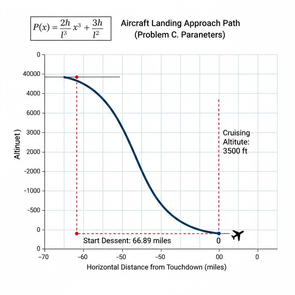
We define the origin (0,0) as the touchdown point and the start of descent as (-l, h).
To make the transition seamless, we impose four conditions:
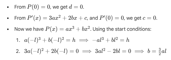
- Touchdown position: P(0) = 0
- Touchdown slope: P'(0) = 0 (The plane should be level with the runway at the moment of contact).
- Starting position: P(-l) = h
- Starting slope: P'(-l) = 0 (The plane is flying level at cruising altitude before it begins to drop).
Solving for coefficients:
Substitute b into the first equation:
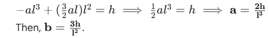
The polynomial is:
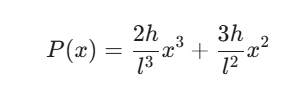
B. Relating Acceleration to the Constant k
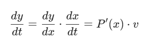
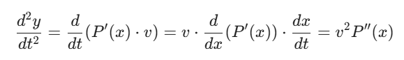
To find vertical acceleration, we need to look at the vertical position y with respect to time t.
Given constant horizontal speed v, we know x = vt – l (starting at distance l). Thus, dx / dt = v.
Using the Chain Rule for vertical velocity:
Now, find vertical acceleration (d2y / dt2):
Find P”(x):
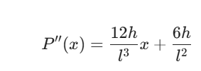
The maximum absolute value of P”(x) on the interval [-l, 0] occurs at the endpoints x=0 or x=-l, where |P”(x)| = 6h / l2.
Substituting this into our acceleration equation:
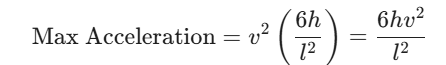
Since this must not exceed k:
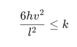
C. Calculating the Descent Distance
Given Data:
- k = 800 mi/hr2
- v = 300 mi/hr
- h = 35,000 ft
First, we must convert h to miles so the units match:
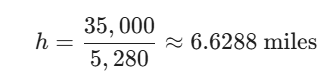
Using the inequality from Part B, we solve for l:
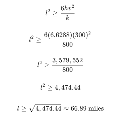
Result: The pilot should start the descent approximately 67 miles away from the airport.
What are related rates?
Related Rates problems involve finding the rate at which one quantity changes by relating it to other quantities whose rates of change are already known.
This is the practical application of the Chain Rule. If two variables (like the radius and volume of a balloon) are linked by an equation, their derivatives with respect to time (t) are also linked.
1. The Core Concept
Imagine you are filling a spherical balloon with air. As you pump air in at a constant rate:
- The Volume (V) increases.
- The Radius (r) increases.
- The Surface Area (S) increases.
Even though you are only controlling the volume, the radius and surface area “relatedly” change. However, they don’t change at the same speed. As the balloon gets bigger, the radius actually starts growing more slowly even if you pump air at the same speed.
2. The Step-by-Step Method
To solve a related rates problem, follow this standard procedure:
- Identify the Variables: List the known rates (e.g., dV / dt = 2 cm3/s) and the rate you need to find (e.g., dr / dt = ?).
- Find the Equation: Write a formula that connects the variables (e.g., V = 4 / 3πr3 for a sphere).
- Differentiate with respect to Time (t): Use implicit differentiation. Every variable is treated as a function of time.
- Example:
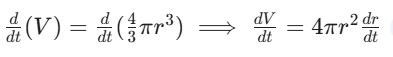
- Substitute and Solve: Plug in the specific values for that exact moment in time to solve for the unknown rate.
3. Classic Examples
The Sliding Ladder
A ladder leans against a wall. If the bottom of the ladder slides away from the wall at a constant speed, how fast is the top sliding down?
- Relationship: The Pythagorean Theorem (x2 + y2 = L2).
- Rate Logic: As x increases, y must decrease to keep L (the ladder length) constant.
The Filling Conical Tank
Water is poured into a cone-shaped tank. Because the cone gets wider at the top, the water level rises quickly at the bottom but slows down as the tank fills.
- Relationship: Volume of a cone (V = (1 / 3)πr2h).
- Complexity: You often use similar triangles to relate r and h so you only have one variable to differentiate.
4. Why it Matters
Related rates are essential in engineering and safety. For example:
- Air Traffic Control: Calculating the rate at which the distance between two planes is changing to prevent collisions.
- Oil Spills: Predicting how fast the radius of a circular spill is expanding based on the rate of the leak.
- Medicine: Monitoring the rate at which a tumor’s volume is changing based on its diameter in a scan.
Key Rule: Never plug in the “static” numbers (like “the radius is 5”) until after you have differentiated. If you plug them in too early, the derivative will incorrectly come out to zero!
What are linear approximations and differentials?
Linear approximation is the mathematical equivalent of “zooming in” on a curve until it looks like a straight line. Because straight lines are much easier to calculate than complex curves, we use the tangent line to estimate the value of a function near a specific point.
1. The Tangent Line Approximation
If you have a complicated function f(x), and you know its value and slope at a point a, the equation of the tangent line at that point is:
L(x) = f(a) + f'(a)(x – a)
- L(x) is the “Linearization” of the function.
- f(a) is the starting height.
- f'(a)(x – a) is the “slope times distance,” which tells you how much the height has changed.
Why use it?
Imagine trying to calculate √4.1 without a calculator.
- You know √4 = 2.
- The derivative of √x is 1 / 2√x. At x=4, the slope is 1 / 4.
- The “nudge” from 4 to 4.1 is 0.1.
- Estimate: 2 + (1 / 4* 0.1) = 2.025. (The actual value is 2.0248…, so the approximation is incredibly close!)
2. Differentials
Differentials (dx and dy) represent the tiny, infinitesimal changes in the variables. While the derivative dy / dx is the ratio of change, the differentials allow us to treat the numerator and denominator as separate pieces.
If y = f(x), then the differential dy is defined as:
dy = f'(x)dx
The Difference between dy and Δy
- Δy: The actual change in the function’s height as you move along the curve.
- dy: The estimated change in height as you move along the tangent line.
As dx gets smaller and smaller, the gap between dy and Δy vanishes.
[Image showing the geometric relationship between dx, dy, and delta y on a graph]
3. Real-World Application: Error Propagation
In science and engineering, no measurement is perfect. Differentials help us calculate how a small error in a measurement (like the radius of a piston) affects the final calculation (like the volume of the engine).
Example: If you measure the side of a square cube with a possible error of dx, the error in the volume (V = x3) is estimated by:
dV = 3x2 dx
Summary of Terms
| Term | Notation | Description |
| Linearization | L(x) | The equation of the tangent line used as a “local” proxy for the function. |
| Independent Differential | dx | A small change in the input variable x. |
| Dependent Differential | dy | The change in y along the tangent line. |
| Propagated Error | dy or dV | How an input error “travels” through a formula to the result. |
What are Taylor Polynomials?
A Taylor Polynomial is essentially a “super-powered” version of the linear approximation we just discussed.
While a linear approximation uses a straight line (a 1st-degree polynomial) to mimic a curve at a specific point, a Taylor Polynomial uses higher-degree terms (x2, x3, x4, etc.) to “bend” the approximation so it stays hugged against the original curve for a much longer distance.
1. The Core Idea: Matching Derivatives
To make a polynomial P(x) look like a function f(x) at a specific point a, we force them to share the same “DNA.” We design the polynomial so that at point a:
- The heights are the same: P(a) = f(a)
- The slopes are the same: P'(a) = f'(a)
- The curvatures are the same: P”(a) = f”(a)
- The “jerks” are the same: P”'(a) = f”'(a)
The more derivatives you match, the more accurate the polynomial becomes.
2. The General Formula
The Taylor Polynomial of degree n for a function f centered at point a is:
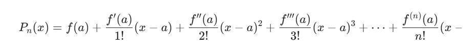
- (x-a)n: This shifts the polynomial so it is centered at a.
- n! (Factorial): This is the “secret sauce.” It accounts for the power rule being applied multiple times during differentiation, keeping the coefficients balanced.
Note: When the center a = 0, the polynomial is specifically called a Maclaurin Polynomial.
3. Why are they useful?
Calculators and computers don’t actually “know” what sin(x) or ex is. They only know how to do basic arithmetic (addition, subtraction, multiplication, division).
When you type sin(0.5) into a calculator, it uses a Taylor Polynomial to turn that trig function into a simple string of arithmetic:
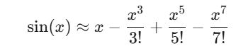
[Image comparing the graph of e^x with its 2nd and 3rd degree Maclaurin polynomials]
4. Convergence and “The Tail”
Taylor Polynomials are excellent locally (near the center a), but as you move further away, the polynomial eventually “breaks” and flies away from the original curve.
The difference between the actual function and the polynomial is called the Remainder ($R_n$). In advanced calculus, we use Taylor’s Theorem to prove that as n goes to infinity, the remainder goes to zero for many common functions. At that point, the polynomial becomes a Taylor Series.
Summary: Polynomial vs. Series
- Taylor Polynomial: A finite sum (e.g., up to x3). It is an approximation.
- Taylor Series: An infinite sum. For many functions, it is exactly equal to the function.