
The area problem is one of the two central pillars of calculus (the other being the tangent line problem). At its heart, it asks a deceptively simple question: How can we calculate the exact area of a region with curved boundaries?
While we have simple formulas for the area of a rectangle (A = lw) or a triangle (A = (1 / 2) bh), those formulas fail when the “top” of the shape is defined by a changing function, such as f(x) = x2.
The Strategy: Exhaustion and Summation
To solve this, calculus uses a “divide and conquer” strategy. Since we already know how to find the area of a rectangle, we fill the space under the curve with a series of thin rectangles.
- Approximation: We divide the interval on the x-axis into n sub-intervals.
- Rectangles: We draw a rectangle in each interval. The height of each rectangle is determined by the value of the function f(x) at that point.
- Summation: We add up the areas of all these rectangles. This is known as a Riemann Sum.
The Leap to Calculus: The Limit
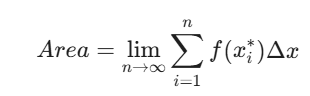
The sum of the rectangles is just an estimate. If the rectangles are wide, you’ll have “gaps” or “overlaps” that make the calculation inaccurate. However, as you make the rectangles thinner and increase the number of rectangles ($n$), the approximation becomes more precise.
The “Area Problem” is officially solved by taking the limit as the number of rectangles approaches infinity:
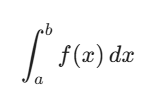
This limit is what we define as the Definite Integral:
Why It Matters
The solution to the area problem isn’t just about geometry. In physics and data science, “area under the curve” represents accumulation. For example:
- The area under a velocity-time graph gives you the total distance traveled.
- The area under a marginal cost curve gives you the total cost.
The Big Twist
The most elegant part of this story is the Fundamental Theorem of Calculus, which discovered that you don’t actually have to sum up infinite rectangles manually. Instead, you can find the area simply by using the inverse of a derivative (the antiderivative).